
Python: two examples
Utilizzo l’environment conda py3
1
~$ conda activate py3
Versione modulo installato
1
2
3
4
5
6
7
8
9
10
11
~$ pip show pandas_datareader
Name: pandas-datareader
Version: 0.9.0
Summary: Data readers extracted from the pandas codebase,should be compatible with recent pandas versions
Home-page: https://github.com/pydata/pandas-datareader
Author: The PyData Development Team
Author-email: pydata@googlegroups.com
License: BSD License
Location: /home/user/miniconda3/envs/py3/lib/python3.7/site-packages
Requires: requests, pandas, lxml
Required-by:
Indice
Due laboratori
911 Calls Project
Kaggle data
1
2
3
4
5
6
7
import numpy as np
import pandas as pd

import matplotlib.pyplot as plt
import seaborn as sns

%matplotlib inline
1
2
3
# import df
df = pd.read_csv('911.csv')
df.head()
| lat | lng | desc | zip | title | timeStamp | twp | addr | e | |
|---|---|---|---|---|---|---|---|---|---|
| 0 | 40.297876 | -75.581294 | REINDEER CT & DEAD END; NEW HANOVER; Station ... | 19525.0 | EMS: BACK PAINS/INJURY | 2015-12-10 17:40:00 | NEW HANOVER | REINDEER CT & DEAD END | 1 |
| 1 | 40.258061 | -75.264680 | BRIAR PATH & WHITEMARSH LN; HATFIELD TOWNSHIP... | 19446.0 | EMS: DIABETIC EMERGENCY | 2015-12-10 17:40:00 | HATFIELD TOWNSHIP | BRIAR PATH & WHITEMARSH LN | 1 |
| 2 | 40.121182 | -75.351975 | HAWS AVE; NORRISTOWN; 2015-12-10 @ 14:39:21-St... | 19401.0 | Fire: GAS-ODOR/LEAK | 2015-12-10 17:40:00 | NORRISTOWN | HAWS AVE | 1 |
| 3 | 40.116153 | -75.343513 | AIRY ST & SWEDE ST; NORRISTOWN; Station 308A;... | 19401.0 | EMS: CARDIAC EMERGENCY | 2015-12-10 17:40:01 | NORRISTOWN | AIRY ST & SWEDE ST | 1 |
| 4 | 40.251492 | -75.603350 | CHERRYWOOD CT & DEAD END; LOWER POTTSGROVE; S... | NaN | EMS: DIZZINESS | 2015-12-10 17:40:01 | LOWER POTTSGROVE | CHERRYWOOD CT & DEAD END | 1 |
1
df.info()
1
2
3
4
5
6
7
8
9
10
11
12
13
14
15
16
<class 'pandas.core.frame.DataFrame'>
RangeIndex: 99492 entries, 0 to 99491
Data columns (total 9 columns):
 #   Column     Non-Null Count  Dtype
---  ------     --------------  -----
 0   lat        99492 non-null  float64
 1   lng        99492 non-null  float64
 2   desc       99492 non-null  object
 3   zip        86637 non-null  float64
 4   title      99492 non-null  object
 5   timeStamp  99492 non-null  object
 6   twp        99449 non-null  object
 7   addr       98973 non-null  object
 8   e          99492 non-null  int64
dtypes: float64(3), int64(1), object(5)
memory usage: 6.8+ MB
1
2
# top 5 zipcode for 911 cals
df['zip'].value_counts().head()
1
2
3
4
5
6
19401.0    6979
19464.0    6643
19403.0    4854
19446.0    4748
19406.0    3174
Name: zip, dtype: int64
1
2
# top 5 townships (twp) for 911 calls
df['twp'].value_counts().head()
1
2
3
4
5
6
LOWER MERION    8443
ABINGTON        5977
NORRISTOWN      5890
UPPER MERION    5227
CHELTENHAM      4575
Name: twp, dtype: int64
1
2
3
# unique title codes
# len(df['title'].unique())
df['title'].nunique()
1
110
1
2
# 'Reasons/Departments' extraction from title
df['Reason'] = df['title'].apply(lambda x: x.split(':')[0])
1
2
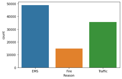
# frequency table of 'Reasons/Departments'
df['Reason'].value_counts()
1
2
3
4
EMS        48877
Traffic    35695
Fire       14920
Name: Reason, dtype: int64
1
2
# countplot with seaborn
sns.countplot(x='Reason', data=df)
1
<matplotlib.axes._subplots.AxesSubplot at 0x7ff700edb9d0>
1
2
# timeStamp
df['timeStamp'][0]
1
'2015-12-10 17:40:00'
1
2
# data type of the objects in the timeStamp column
type(df['timeStamp'][0])
1
str
1
2
3
# convert timeStamp string to DateTime
df['timeStamp'] = pd.to_datetime(df['timeStamp'])
df['timeStamp'][0]
1
Timestamp('2015-12-10 17:40:00')
1
2
# assegno la prima osservazione, così posso usare shift+tab nella cella successiva per vedere i methods
ora = df['timeStamp'][0]
1
2
# estraggo l'ora
ora.hour
1
17
1
2
3
4
# costruisco variabile ora, mese e giorno della settimana
df['Hour'] = df['timeStamp'].apply(lambda x: x.hour)
df['Month'] = df['timeStamp'].apply(lambda x: x.month)
df['Day of Week'] = df['timeStamp'].apply(lambda x: x.dayofweek)
1
2
3
# mapping number day week to day week
dmap = {0:'Mon',1:'Tue',2:'Wed',3:'Thu',4:'Fri',5:'Sat',6:'Sun'}
df['Day of Week'] = df['Day of Week'].map(dmap)
1
2
3
4
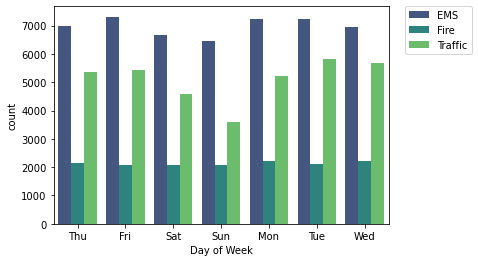
# countplot day week
sns.countplot(x='Day of Week',data=df,hue='Reason',palette='viridis')
# plt.legend(loc='center left', bbox_to_anchor=(1.0, 0.5))
plt.legend(bbox_to_anchor=(1.05, 1), loc=2, borderaxespad=0.)
1
<matplotlib.legend.Legend at 0x7ff6fffce450>
1
2
3
4
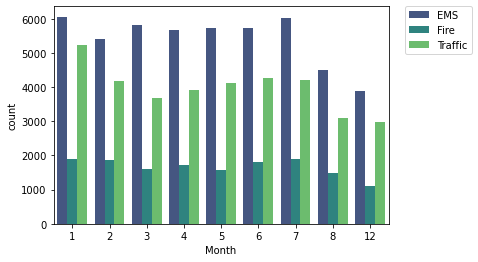
# countplot month
sns.countplot(x='Month',data=df,hue='Reason',palette='viridis')
# plt.legend(loc='center left', bbox_to_anchor=(1.0, 0.5))
plt.legend(bbox_to_anchor=(1.05, 1), loc=2, borderaxespad=0.)
1
<matplotlib.legend.Legend at 0x7ff6ff24ea50>
1
# 9-10-11 months missing
1
2
# attenzione sono presenti dei missing, non usare le colonne con i missing per i conteggi
df.isnull().sum()
1
2
3
4
5
6
7
8
9
10
11
12
13
14
lat                0
lng                0
desc               0
zip            12855
title              0
timeStamp          0
twp               43
addr             519
e                  0
Reason             0
Hour               0
Month              0
Day of Week        0
dtype: int64
1
2
# attenzione sono presenti dei missing, non usare le colonne con i missing per i conteggi
df.isnull().any()
1
2
3
4
5
6
7
8
9
10
11
12
13
14
lat            False
lng            False
desc           False
zip             True
title          False
timeStamp      False
twp             True
addr            True
e              False
Reason         False
Hour           False
Month          False
Day of Week    False
dtype: bool
1
2
3
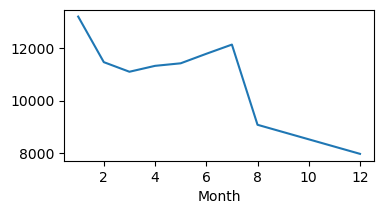
# groupby month
byMonth = df.groupby(by='Month').count()
byMonth.head()
| lat | lng | desc | zip | title | timeStamp | twp | addr | e | Reason | Hour | Day of Week | |
|---|---|---|---|---|---|---|---|---|---|---|---|---|
| Month | ||||||||||||
| 1 | 13205 | 13205 | 13205 | 11527 | 13205 | 13205 | 13203 | 13096 | 13205 | 13205 | 13205 | 13205 |
| 2 | 11467 | 11467 | 11467 | 9930 | 11467 | 11467 | 11465 | 11396 | 11467 | 11467 | 11467 | 11467 |
| 3 | 11101 | 11101 | 11101 | 9755 | 11101 | 11101 | 11092 | 11059 | 11101 | 11101 | 11101 | 11101 |
| 4 | 11326 | 11326 | 11326 | 9895 | 11326 | 11326 | 11323 | 11283 | 11326 | 11326 | 11326 | 11326 |
| 5 | 11423 | 11423 | 11423 | 9946 | 11423 | 11423 | 11420 | 11378 | 11423 | 11423 | 11423 | 11423 |
1
2
3
4
# line plot count, è evidente la caduta causata dal dato mancante
plt.figure(figsize=(4,2),dpi=100)
plt.style.use('default')
byMonth['lat'].plot()
1
<matplotlib.axes._subplots.AxesSubplot at 0x7ff703e0eed0>
1
2
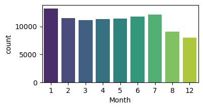
3
# count plot, è evidente la caduta causata dal dato mancante
plt.figure(figsize=(4,2),dpi=100)
sns.countplot(x='Month',data=df,palette='viridis')
1
<matplotlib.axes._subplots.AxesSubplot at 0x7ff6ff5d5c50>
1
2
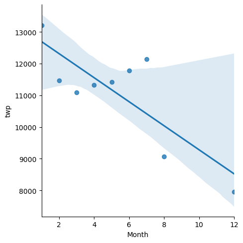
3
# linear fit calls per month
# trasformo l'index month in una colonna così da poterlo usare come variabile x
sns.lmplot(x='Month',y='twp',data=byMonth.reset_index())
1
<seaborn.axisgrid.FacetGrid at 0x7ff6ff5a60d0>
1
2
3
# creo colonna data da timeStamp
df['Date'] = df['timeStamp'].apply(lambda x: x.date())
df['Date'].head()
1
2
3
4
5
6
0    2015-12-10
1    2015-12-10
2    2015-12-10
3    2015-12-10
4    2015-12-10
Name: Date, dtype: object
1
2
3
4
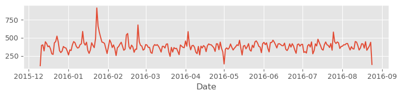
5
# line plot time
plt.figure(figsize=(8,2),dpi=100)
plt.style.use('ggplot') # plt.style.use('default')
df.groupby(by='Date').count()['twp'].plot()
plt.tight_layout()
1
2
3
4
5
6
7
8
9
10
11
12
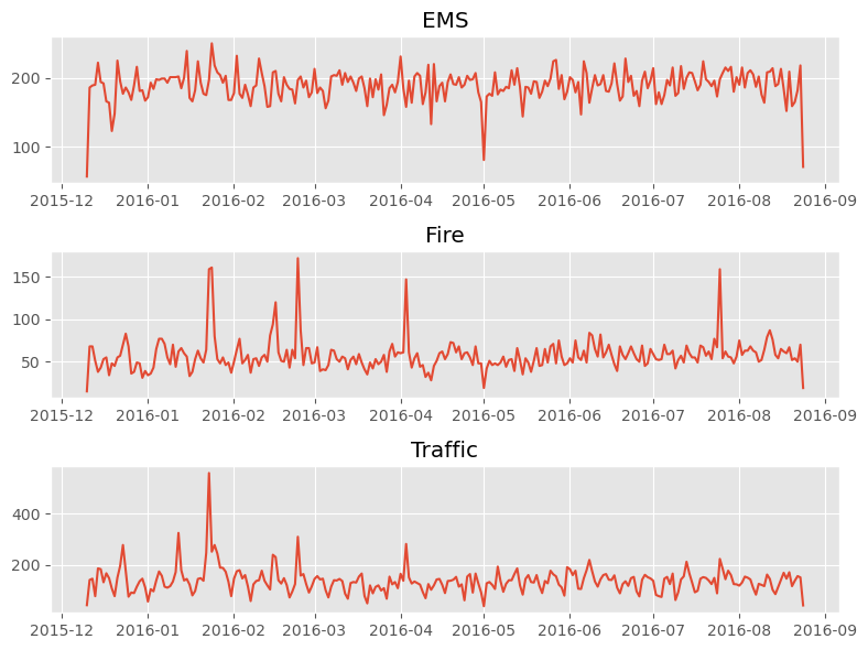
13
# plot per ogni Reason
fig,axes = plt.subplots(nrows=3,ncols=1,figsize=(8,6))
axes[0].plot(df[df['Reason']=='EMS'].groupby(by='Date').count()['twp'])
axes[0].set_title('EMS')
axes[1].plot(df[df['Reason']=='Fire'].groupby(by='Date').count()['twp'])
axes[1].set_title('Fire')
axes[2].plot(df[df['Reason']=='Traffic'].groupby(by='Date').count()['twp'])
axes[2].set_title('Traffic')
plt.tight_layout()
1
2
3
# heatmap column Hours & Index Day of the Week (prepare data - metodo 1)
dayHour = df[['Day of Week','Hour']].pivot_table(index='Day of Week',columns='Hour',values='Day of Week',aggfunc=len)
dayHour
| Hour | 0 | 1 | 2 | 3 | 4 | 5 | 6 | 7 | 8 | 9 | ... | 14 | 15 | 16 | 17 | 18 | 19 | 20 | 21 | 22 | 23 |
|---|---|---|---|---|---|---|---|---|---|---|---|---|---|---|---|---|---|---|---|---|---|
| Day of Week | |||||||||||||||||||||
| Fri | 275 | 235 | 191 | 175 | 201 | 194 | 372 | 598 | 742 | 752 | ... | 932 | 980 | 1039 | 980 | 820 | 696 | 667 | 559 | 514 | 474 |
| Mon | 282 | 221 | 201 | 194 | 204 | 267 | 397 | 653 | 819 | 786 | ... | 869 | 913 | 989 | 997 | 885 | 746 | 613 | 497 | 472 | 325 |
| Sat | 375 | 301 | 263 | 260 | 224 | 231 | 257 | 391 | 459 | 640 | ... | 789 | 796 | 848 | 757 | 778 | 696 | 628 | 572 | 506 | 467 |
| Sun | 383 | 306 | 286 | 268 | 242 | 240 | 300 | 402 | 483 | 620 | ... | 684 | 691 | 663 | 714 | 670 | 655 | 537 | 461 | 415 | 330 |
| Thu | 278 | 202 | 233 | 159 | 182 | 203 | 362 | 570 | 777 | 828 | ... | 876 | 969 | 935 | 1013 | 810 | 698 | 617 | 553 | 424 | 354 |
| Tue | 269 | 240 | 186 | 170 | 209 | 239 | 415 | 655 | 889 | 880 | ... | 943 | 938 | 1026 | 1019 | 905 | 731 | 647 | 571 | 462 | 274 |
| Wed | 250 | 216 | 189 | 209 | 156 | 255 | 410 | 701 | 875 | 808 | ... | 904 | 867 | 990 | 1037 | 894 | 686 | 668 | 575 | 490 | 335 |
7 rows × 24 columns
1
2
3
# heatmap column Hours & Index Day of the Week (prepare data - metodo 2)
dayHour = df.groupby(by=['Day of Week','Hour']).count()['Reason'].unstack(level=-1)
dayHour
| Hour | 0 | 1 | 2 | 3 | 4 | 5 | 6 | 7 | 8 | 9 | ... | 14 | 15 | 16 | 17 | 18 | 19 | 20 | 21 | 22 | 23 |
|---|---|---|---|---|---|---|---|---|---|---|---|---|---|---|---|---|---|---|---|---|---|
| Day of Week | |||||||||||||||||||||
| Fri | 275 | 235 | 191 | 175 | 201 | 194 | 372 | 598 | 742 | 752 | ... | 932 | 980 | 1039 | 980 | 820 | 696 | 667 | 559 | 514 | 474 |
| Mon | 282 | 221 | 201 | 194 | 204 | 267 | 397 | 653 | 819 | 786 | ... | 869 | 913 | 989 | 997 | 885 | 746 | 613 | 497 | 472 | 325 |
| Sat | 375 | 301 | 263 | 260 | 224 | 231 | 257 | 391 | 459 | 640 | ... | 789 | 796 | 848 | 757 | 778 | 696 | 628 | 572 | 506 | 467 |
| Sun | 383 | 306 | 286 | 268 | 242 | 240 | 300 | 402 | 483 | 620 | ... | 684 | 691 | 663 | 714 | 670 | 655 | 537 | 461 | 415 | 330 |
| Thu | 278 | 202 | 233 | 159 | 182 | 203 | 362 | 570 | 777 | 828 | ... | 876 | 969 | 935 | 1013 | 810 | 698 | 617 | 553 | 424 | 354 |
| Tue | 269 | 240 | 186 | 170 | 209 | 239 | 415 | 655 | 889 | 880 | ... | 943 | 938 | 1026 | 1019 | 905 | 731 | 647 | 571 | 462 | 274 |
| Wed | 250 | 216 | 189 | 209 | 156 | 255 | 410 | 701 | 875 | 808 | ... | 904 | 867 | 990 | 1037 | 894 | 686 | 668 | 575 | 490 | 335 |
7 rows × 24 columns
1
2
3
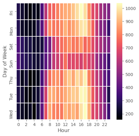
# heatmap column Hours & Index Day of the Week
plt.figure(figsize=(5,5))
sns.heatmap(dayHour,cmap='magma',linecolor='white',linewidths=1)
1
<matplotlib.axes._subplots.AxesSubplot at 0x7ff6ff321a90>
1
2
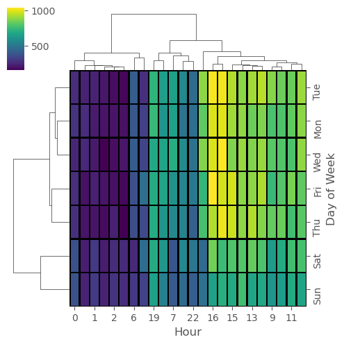
# clustermap column Hours & Index Day of the Week
sns.clustermap(dayHour,cmap='viridis',linecolor='black',linewidths=1,figsize=(5,5))
1
<seaborn.matrix.ClusterGrid at 0x7ff6feffc690>
1
2
3
4
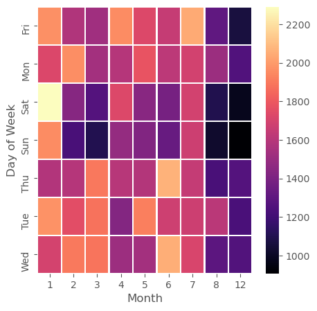
# heatmap column Hours & Index Day of the Week
dayMonth = df.groupby(by=['Day of Week','Month']).count()['Reason'].unstack(level=-1)
plt.figure(figsize=(5,5))
sns.heatmap(dayMonth,cmap='magma',linecolor='white',linewidths=1)
1
<matplotlib.axes._subplots.AxesSubplot at 0x7ff6fe48b310>
1
2
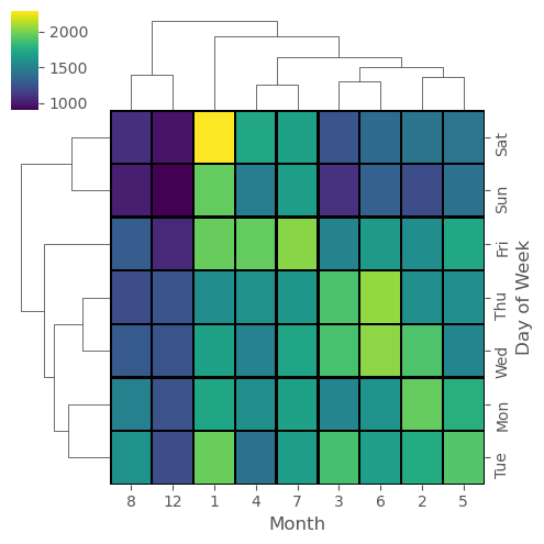
# clustermap column Month & Index Day of the Week
sns.clustermap(dayMonth,cmap='viridis',linecolor='black',linewidths=1,figsize=(5,5))
1
<seaborn.matrix.ClusterGrid at 0x7ff6fe3ba150>
Finance Project
Read data from Google finance with pandas-datareader
Documentazione pandas-datareader remote_data
1
2
3
4
5
6
7
8
9
10
from pandas_datareader import data, wb

import pandas as pd
import numpy as np
import datetime

import matplotlib.pyplot as plt
import seaborn as sns

%matplotlib inline
Aggiunta 16/04/2021
Per scaricare indici di borsa torna comodo yfinance che ha una granularità anche del minuto ma con un limite di download massimo di 7 giorni.
1
2
3
4
5
6
7
8
9
10
11
12
13
14
15
16
17
18
19
20
21
import yfinance as yf
import datetime
FTSEMIB = yf.download(tickers="FTSEMIB.MI",
            start=datetime.datetime(2021, 4, 14),
            end=datetime.datetime(2021, 4, 16),
            interval="1m").sort_values(by='Datetime', ascending=False).head()

NASDAQ = yf.download(tickers="^IXIC",
            start=datetime.datetime(2021, 4, 14),
            end=datetime.datetime(2021, 4, 16),
            interval="1m").sort_values(by='Datetime', ascending=False).head()

BITCOIN_USD = yf.download(tickers="BTC-USD",
                          start=datetime.datetime(2021, 4, 14),
                          end=datetime.datetime(2021, 4, 16),
                          interval="1m").sort_values(by='Datetime', ascending=False).head()

TESLA = yf.download(tickers="TSLA",
                    start=datetime.datetime(2021, 4, 14),
                    end=datetime.datetime(2021, 4, 16),
                    interval="1m").sort_values(by='Datetime', ascending=False).head()
Riprendendo l’esercitazione..
1
2
3
4
5
6
7
8
9
10
11
12
13
14
15
# download data
start = datetime.datetime(2006, 1, 1)
end = datetime.datetime(2016, 1, 1)
BAC = data.DataReader('BAC', 'yahoo', start, end) # Bank of America
C = data.DataReader('C', 'yahoo', start, end)     # CitiGroup
GS = data.DataReader('GS', 'yahoo', start, end)   # Goldman Sachs
JPM = data.DataReader('JPM', 'yahoo', start, end) # JPMorgan Chase
MS = data.DataReader('MS', 'yahoo', start, end)   # Morgan Stanley
WFC = data.DataReader('WFC', 'yahoo', start, end) # Wells Fargo

# per scaricarli tutti in un comando
# df = data.DataReader(['BAC', 'C', 'GS', 'JPM', 'MS', 'WFC'],'yahoo', start, end)

# nel caso in cui non vada l'import (nb. qui CitiGroup presenta un dato anomalo eccessivo 'Stock Split C')
# df = pd.read_pickle('all_banks')
1
2
3
# lista delle sigle banche ordinata
tickers = sorted(['C', 'BAC','JPM','GS','MS','WFC'])
tickers
1
['BAC', 'C', 'GS', 'JPM', 'MS', 'WFC']
1
2
3
# creo df unico
bank_stocks = pd.concat([BAC, C, GS, JPM, MS, WFC],axis=1,keys=tickers)
bank_stocks.head()
| BAC | C | ... | MS | WFC | |||||||||||||||||
|---|---|---|---|---|---|---|---|---|---|---|---|---|---|---|---|---|---|---|---|---|---|
| High | Low | Open | Close | Volume | Adj Close | High | Low | Open | Close | ... | Open | Close | Volume | Adj Close | High | Low | Open | Close | Volume | Adj Close | |
| Date | |||||||||||||||||||||
| 2006-01-03 | 47.180000 | 46.150002 | 46.919998 | 47.080002 | 16296700.0 | 35.054218 | 493.799988 | 481.100006 | 490.000000 | 492.899994 | ... | 57.169998 | 58.310001 | 5377000.0 | 37.399338 | 31.975000 | 31.195000 | 31.600000 | 31.900000 | 11016400.0 | 20.408512 |
| 2006-01-04 | 47.240002 | 46.450001 | 47.000000 | 46.580002 | 17757900.0 | 34.681938 | 491.000000 | 483.500000 | 488.600006 | 483.799988 | ... | 58.700001 | 58.349998 | 7977800.0 | 37.424999 | 31.820000 | 31.365000 | 31.799999 | 31.530001 | 10870000.0 | 20.171795 |
| 2006-01-05 | 46.830002 | 46.320000 | 46.580002 | 46.639999 | 14970700.0 | 34.726604 | 487.799988 | 484.000000 | 484.399994 | 486.200012 | ... | 58.549999 | 58.509998 | 5778000.0 | 37.527611 | 31.555000 | 31.309999 | 31.500000 | 31.495001 | 10158000.0 | 20.149401 |
| 2006-01-06 | 46.910000 | 46.349998 | 46.799999 | 46.570000 | 12599800.0 | 34.674480 | 489.000000 | 482.000000 | 488.799988 | 486.200012 | ... | 58.770000 | 58.570000 | 6889800.0 | 37.566090 | 31.775000 | 31.385000 | 31.580000 | 31.680000 | 8403800.0 | 20.267757 |
| 2006-01-09 | 46.970001 | 46.360001 | 46.720001 | 46.599998 | 15619400.0 | 34.696808 | 487.399994 | 483.000000 | 486.000000 | 483.899994 | ... | 58.630001 | 59.189999 | 4144500.0 | 37.963749 | 31.825001 | 31.555000 | 31.674999 | 31.674999 | 5619600.0 | 20.264565 |
5 rows × 36 columns
1
2
3
# definisco i nomi colonna del multilevel df
bank_stocks.columns.names = ['Bank Ticker','Stock Info']
bank_stocks.columns.names
1
FrozenList(['Bank Ticker', 'Stock Info'])
EDA (Exploratory Data Analysis)
Documentazione Multi-Level Indexing and Cross Section
1
bank_stocks.head()
| Bank Ticker | BAC | C | ... | MS | WFC | ||||||||||||||||
|---|---|---|---|---|---|---|---|---|---|---|---|---|---|---|---|---|---|---|---|---|---|
| Stock Info | High | Low | Open | Close | Volume | Adj Close | High | Low | Open | Close | ... | Open | Close | Volume | Adj Close | High | Low | Open | Close | Volume | Adj Close |
| Date | |||||||||||||||||||||
| 2006-01-03 | 47.180000 | 46.150002 | 46.919998 | 47.080002 | 16296700.0 | 35.054218 | 493.799988 | 481.100006 | 490.000000 | 492.899994 | ... | 57.169998 | 58.310001 | 5377000.0 | 37.399338 | 31.975000 | 31.195000 | 31.600000 | 31.900000 | 11016400.0 | 20.408512 |
| 2006-01-04 | 47.240002 | 46.450001 | 47.000000 | 46.580002 | 17757900.0 | 34.681938 | 491.000000 | 483.500000 | 488.600006 | 483.799988 | ... | 58.700001 | 58.349998 | 7977800.0 | 37.424999 | 31.820000 | 31.365000 | 31.799999 | 31.530001 | 10870000.0 | 20.171795 |
| 2006-01-05 | 46.830002 | 46.320000 | 46.580002 | 46.639999 | 14970700.0 | 34.726604 | 487.799988 | 484.000000 | 484.399994 | 486.200012 | ... | 58.549999 | 58.509998 | 5778000.0 | 37.527611 | 31.555000 | 31.309999 | 31.500000 | 31.495001 | 10158000.0 | 20.149401 |
| 2006-01-06 | 46.910000 | 46.349998 | 46.799999 | 46.570000 | 12599800.0 | 34.674480 | 489.000000 | 482.000000 | 488.799988 | 486.200012 | ... | 58.770000 | 58.570000 | 6889800.0 | 37.566090 | 31.775000 | 31.385000 | 31.580000 | 31.680000 | 8403800.0 | 20.267757 |
| 2006-01-09 | 46.970001 | 46.360001 | 46.720001 | 46.599998 | 15619400.0 | 34.696808 | 487.399994 | 483.000000 | 486.000000 | 483.899994 | ... | 58.630001 | 59.189999 | 4144500.0 | 37.963749 | 31.825001 | 31.555000 | 31.674999 | 31.674999 | 5619600.0 | 20.264565 |
5 rows × 36 columns
1
2
# Close price massimo per ciascuna banca
bank_stocks.xs(key='Close',level='Stock Info',axis=1).max()
1
2
3
4
5
6
7
8
Bank Ticker
BAC     54.900002
C      564.099976
GS     247.919998
JPM     70.080002
MS      89.300003
WFC     58.520000
dtype: float64
Formula rendimenti \(r_t = \frac{p_t - p_{t-1}}{p_{t-1}} = \frac{p_t}{p_{t-1}} - 1\)
1
2
3
4
5
6
7
8
# calcolo dei Rendimenti
returns = bank_stocks.xs(key='Close',level='Stock Info',axis=1).pct_change()
returns.columns = returns.columns+' Return'
# returns = pd.DataFrame()
# for tick in tickers:
#     returns[tick+' Return'] = bank_stocks[tick]['Close'].pct_change()

returns.head()
| Bank Ticker | BAC Return | C Return | GS Return | JPM Return | MS Return | WFC Return |
|---|---|---|---|---|---|---|
| Date | ||||||
| 2006-01-03 | NaN | NaN | NaN | NaN | NaN | NaN |
| 2006-01-04 | -0.010620 | -0.018462 | -0.013812 | -0.014183 | 0.000686 | -0.011599 |
| 2006-01-05 | 0.001288 | 0.004961 | -0.000393 | 0.003029 | 0.002742 | -0.001110 |
| 2006-01-06 | -0.001501 | 0.000000 | 0.014169 | 0.007046 | 0.001025 | 0.005874 |
| 2006-01-09 | 0.000644 | -0.004731 | 0.012030 | 0.016242 | 0.010586 | -0.000158 |
1
2
# Citigroup has no 'great' outliers
returns['C Return'].describe()
1
2
3
4
5
6
7
8
9
count    2516.000000
mean       -0.000157
std         0.038672
min        -0.390244
25%        -0.011182
50%        -0.000210
75%         0.010751
max         0.578249
Name: C Return, dtype: float64
1
2
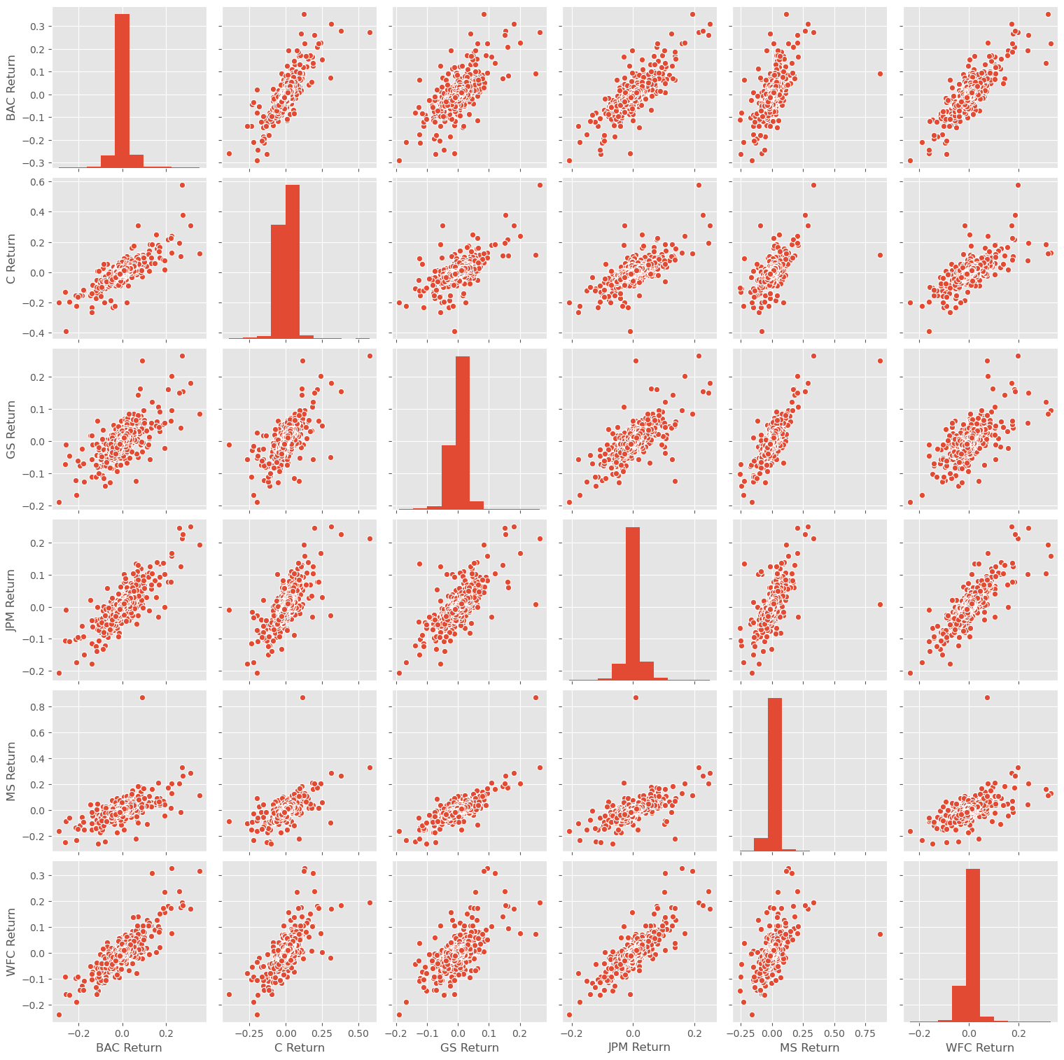
# pairplot
sns.pairplot(returns)
1
<seaborn.axisgrid.PairGrid at 0x7ff6d75a6bd0>
1
2
# Worst Drop (4 of them on Inauguration day)
returns.idxmin()
1
2
3
4
5
6
7
8
Bank Ticker
BAC Return   2009-01-20
C Return     2009-02-27
GS Return    2009-01-20
JPM Return   2009-01-20
MS Return    2008-10-09
WFC Return   2009-01-20
dtype: datetime64[ns]
1
2
# Best Single Day Gain (JPM e MS il migliore poco dopo)
returns.idxmax()
1
2
3
4
5
6
7
8
Bank Ticker
BAC Return   2009-04-09
C Return     2008-11-24
GS Return    2008-11-24
JPM Return   2009-01-21
MS Return    2008-10-13
WFC Return   2008-07-16
dtype: datetime64[ns]
1
2
# standard deviation intero periodo
returns.std()
1
2
3
4
5
6
7
8
Bank Ticker
BAC Return    0.036647
C Return      0.038672
GS Return     0.025390
JPM Return    0.027667
MS Return     0.037819
WFC Return    0.030238
dtype: float64
1
2
3
# standard deviation sul 2015 (filtro o apply con map sull'index)
# returns[returns.index.map(lambda x: x.year)==2015].std()
returns.loc['2015-01-01':'2015-12-31'].std()
1
2
3
4
5
6
7
8
Bank Ticker
BAC Return    0.016163
C Return      0.015289
GS Return     0.014046
JPM Return    0.014017
MS Return     0.016249
WFC Return    0.012591
dtype: float64
1
2
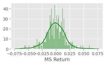
3
# distplot return del 2015 di MS
plt.figure(figsize=(4,2),dpi=100)
sns.distplot(returns.loc['2015-01-01':'2015-12-31']['MS Return'],bins=100,color='green')
1
<matplotlib.axes._subplots.AxesSubplot at 0x7ff6cf835e50>
1
2
3
# distplot return del 2015 di C
plt.figure(figsize=(4,2),dpi=100)
sns.distplot(returns.loc['2008-01-01':'2008-12-31']['C Return'],bins=100,color='red')
1
<matplotlib.axes._subplots.AxesSubplot at 0x7ff6ce6f98d0>

More Visualization
1
2
3
4
5
6
7
8
9
10
import matplotlib.pyplot as plt
import seaborn as sns
sns.set_style('whitegrid')
%matplotlib inline

import plotly
import cufflinks as cf
cf.go_offline()

from IPython.display import Image
1
2
3
# close stock per ogni banca
close = bank_stocks.xs(key='Close',level='Stock Info',axis=1)
close.head()
| Bank Ticker | BAC | C | GS | JPM | MS | WFC |
|---|---|---|---|---|---|---|
| Date | ||||||
| 2006-01-03 | 47.080002 | 492.899994 | 128.869995 | 40.189999 | 58.310001 | 31.900000 |
| 2006-01-04 | 46.580002 | 483.799988 | 127.089996 | 39.619999 | 58.349998 | 31.530001 |
| 2006-01-05 | 46.639999 | 486.200012 | 127.040001 | 39.740002 | 58.509998 | 31.495001 |
| 2006-01-06 | 46.570000 | 486.200012 | 128.839996 | 40.020000 | 58.570000 | 31.680000 |
| 2006-01-09 | 46.599998 | 483.899994 | 130.389999 | 40.669998 | 59.189999 | 31.674999 |
1
2
3
4
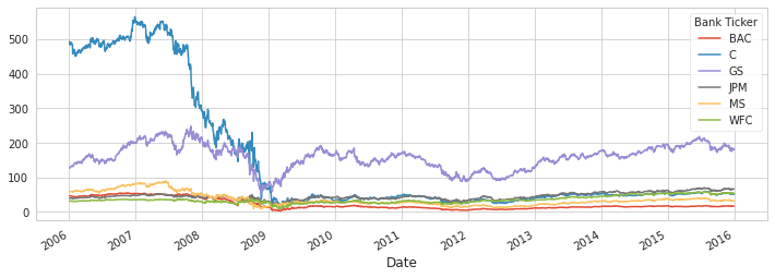
5
# line plot per ogni close stock (matplotlib)
close.plot(figsize=(12,4))
# for tick in tickers:
# bank_stocks[tick]['Close'].plot(figsize=(12,4),label=tick)
# plt.legend()
1
<matplotlib.axes._subplots.AxesSubplot at 0x7ff6df437790>
1
2
3
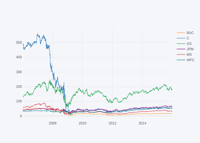
# line plot per ogni close stock (plotly)
fig = close.iplot(asFigure=True)
fig.show()
1
2
3
# display static image
img_bytes = fig.to_image(format="png")
Image(img_bytes)
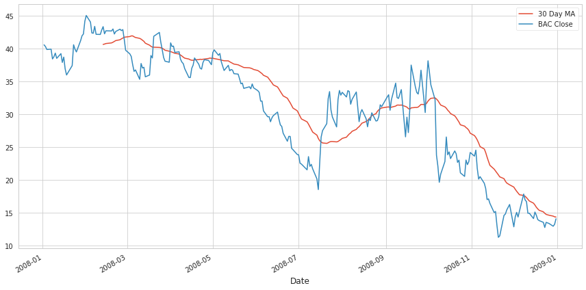
Moving Averages
1
2
3
4
5
6
# close stock BAC e MA 30 giorni
fig = plt.figure(figsize=(12,6))
close.loc['2008-01-01':'2008-12-31']['BAC'].rolling(window=30).mean().plot(label='30 Day MA')
close.loc['2008-01-01':'2008-12-31']['BAC'].plot(label='BAC Close')
plt.legend()
plt.tight_layout()
1
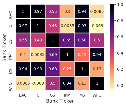
2
3
# heatmap close price (reversescale color)
plt.figure(figsize=(5,4),dpi=100)
sns.heatmap(close.corr(),cmap='magma_r',linecolor='white',linewidths=1,annot=True)
1
<matplotlib.axes._subplots.AxesSubplot at 0x7ff6daa16210>
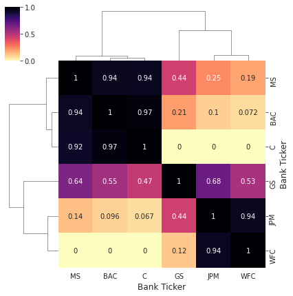
1
2
# clustermap close price
sns.clustermap(close.corr(),standard_scale=1,figsize=(6,6),annot=True,cmap='magma_r')
1
<seaborn.matrix.ClusterGrid at 0x7ff6da90a1d0>
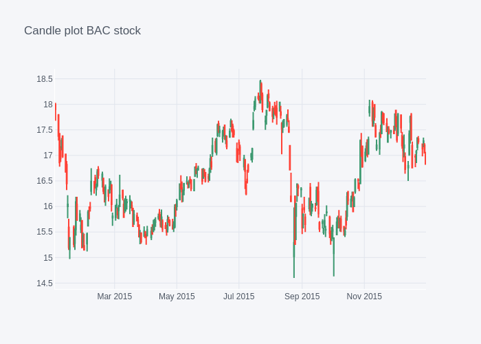
Technical Analysis
1
2
3
# candle plot BAC
fig = BAC[['Open', 'High', 'Low', 'Close']].loc['2015-01-01':'2016-01-01'].iplot(kind='candle',asFigure=True,title='Candle plot BAC stock')
fig.show()
1
2
3
# display static image
img_bytes = fig.to_image(format="png")
Image(img_bytes)
1
2
# Simple Moving Average per MS (da lanciare in locale, non sono riuscito ad esportarla come immagine)
MS['Close'].loc['2015-01-01':'2016-01-01'].ta_plot(study='sma',periods=[13,21,55])
1
2
# Bollinger Band Plot per BAC
BAC['Close'].loc['2015-01-01':'2016-01-01'].ta_plot(study='boll')