Python: Plotly and Choropleth
Utilizzo l’environment conda py3
1
~$ conda activate py3
Versione modulo installato
1
2
3
4
5
6
7
8
9
10
11
~$ pip show chart-studio
Name: chart-studio
Version: 1.1.0
Summary: Utilities for interfacing with plotly's Chart Studio
Home-page: https://plot.ly/python/
Author: Chris P
Author-email: chris@plot.ly
License: MIT
Location: /home/user/miniconda3/envs/py3/lib/python3.7/site-packages
Requires: plotly, requests, retrying, six
Required-by:
Plotly and Choropleth
Per ottenere i grafici interattivi lanciare il codice in locale.
Sono riuscito ad esportarli via web con Markdown solo statici (sono necessari psutil e orca)
1
2
~$ conda install psutil
~$ conda install -c plotly plotly-orca
Cheat sheet Plotly
Documentazione Choropleth
1
2
3
4
5
import chart_studio.plotly as py
import plotly.graph_objs as go
import pandas as pd
from plotly.offline import download_plotlyjs, init_notebook_mode, plot, iplot
from IPython.display import Image
1
2
# per mostrare nel notebook
init_notebook_mode(connected=True)
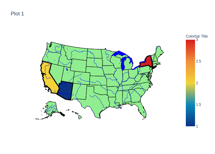
Plot USA-states
1
2
3
4
5
6
7
8
9
10
11
12
13
14
15
16
17
18
19
20
21
22
23
24
25
26
27
28
29
30
31
data = dict(type = 'choropleth',
            locations = ['AZ','CA','NY'],
            locationmode = 'USA-states',
            colorscale= 'Portland',
            text= ['Arizona','Cali','New York'],
            z=[1.0,2.0,3.0],
            marker = dict(line = dict(color = 'rgb(0,0,0)',width = 3)),
            colorbar = {'title':'Colorbar Title'})

layout = dict(title = 'Plot 1')

choromap = go.Figure(data = [data],layout = layout)
choromap.update_geos(
    visible=True,
    resolution=50,
    scope="usa",

    # projection_type="orthographic", # "natural earth"
    # lataxis_showgrid=True, lonaxis_showgrid=True,

    showcoastlines=True, coastlinecolor="RebeccaPurple",
    showland=True, landcolor="LightGreen",
    showocean=True, oceancolor="LightBlue",
    showlakes=True, lakecolor="Blue",
    showrivers=True, rivercolor="Blue",

    showcountries=True, countrycolor="Black",
    showsubunits=True, subunitcolor="Black")
# choromap.show() # si può omettere se si usa il comando precedente
# iplot(choromap) # si può omettere se si usa il comando precedente
# plot(choromap)  # apre in nuova finestra
1
2
# export map
# choromap.write_image("img1.png")
1
2
3
4
# display static image
img_bytes = choromap.to_image(format="png") # parametri: width, height, scale
# img_bytes[:20]
Image(img_bytes)
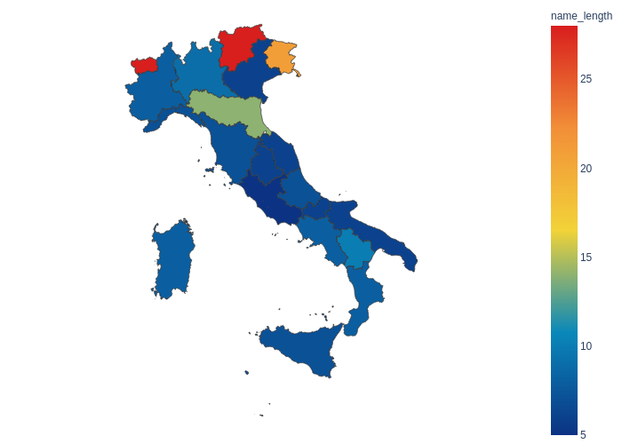
Italy - Regioni
Confini Italiani fonte Openpolis
1
2
3
import pandas as pd
import requests
import plotly.express as px
1
2
3
# carico confini regionali
geojson_url = 'https://raw.githubusercontent.com/AlbGri/AlbGri.github.io/master/assets/files/Openpolis/geojson/limits_IT_regions.geojson'
italy_regions_geo = requests.get(geojson_url).json()
1
2
3
4
5
6
7
8
9
10
# Regioni
regions = ['Piemonte', 'Trentino-Alto Adige/Südtirol', 'Lombardia', 'Puglia', 'Basilicata',
           'Friuli-Venezia Giulia', 'Liguria', "Valle d'Aosta/Vallée d'Aoste", 'Emilia-Romagna',
           'Molise', 'Lazio', 'Veneto', 'Sardegna', 'Sicilia', 'Abruzzo',
           'Calabria', 'Toscana', 'Umbria', 'Campania', 'Marche']
# Create a dataframe with the region names
df = pd.DataFrame(regions, columns=['reg_name'])
# For demonstration, create a column with the length of the region's name
df['name_length'] = df['reg_name'].str.len()
df.head()
| reg_name | name_length | |
|---|---|---|
| 0 | Piemonte | 8 |
| 1 | Trentino-Alto Adige/Südtirol | 28 |
| 2 | Lombardia | 9 |
| 3 | Puglia | 6 |
| 4 | Basilicata | 10 |
1
2
3
4
5
6
7
8
9
10
11
12
# Choropleth representing the length of region names
fig = px.choropleth(data_frame=df,
                    geojson=italy_regions_geo, # anche il geojson_url gli si può passare
                    locations='reg_name',      # name of dataframe column
                    featureidkey='properties.reg_name',  # feature object locations
                    color='name_length',
                    color_continuous_scale="Portland",
                    scope="europe",
                   )
fig.update_geos(showcountries=False, showcoastlines=False, showland=False, fitbounds="locations")
fig.update_layout(margin={"r":0,"t":0,"l":0,"b":0})
# fig.show()
1
2
3
# display static image
img_bytes = fig.to_image(format="png")
Image(img_bytes)
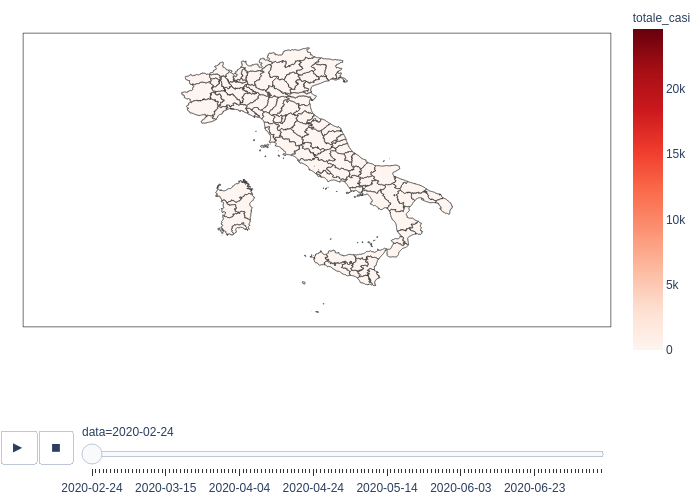
Italy - Province
Confini Italiani fonte Openpolis
Dati COVID-19 fonte Presidenza del Consiglio dei Ministri - Dipartimento della Protezione Civile
1
2
3
4
# from urllib.request import urlopen
import pandas as pd
import plotly.express as px
# import json
1
2
3
4
5
6
# carico confini provinciali
geojson_url = 'https://raw.githubusercontent.com/AlbGri/AlbGri.github.io/master/assets/files/Openpolis/geojson/limits_IT_provinces.geojson'
italy_province_geo = requests.get(geojson_url).json()

# struttura properties (printare tutto il dizionario è pesante)
italy_province_geo['features'][0]['properties']
1
2
3
4
5
6
7
{'prov_name': 'Torino',
 'prov_istat_code_num': 1,
 'prov_acr': 'TO',
 'reg_name': 'Piemonte',
 'reg_istat_code': '01',
 'reg_istat_code_num': 1,
 'prov_istat_code': '001'}
1
2
3
4
# carico df covid
covid_url = 'https://raw.githubusercontent.com/pcm-dpc/COVID-19/master/dati-province/dpc-covid19-ita-province.csv'
df = pd.read_csv(covid_url)
df.head()
| data | stato | codice_regione | denominazione_regione | codice_provincia | denominazione_provincia | sigla_provincia | lat | long | totale_casi | note | |
|---|---|---|---|---|---|---|---|---|---|---|---|
| 0 | 2020-02-24T18:00:00 | ITA | 13 | Abruzzo | 66 | L'Aquila | AQ | 42.351222 | 13.398438 | 0 | NaN |
| 1 | 2020-02-24T18:00:00 | ITA | 13 | Abruzzo | 67 | Teramo | TE | 42.658918 | 13.704400 | 0 | NaN |
| 2 | 2020-02-24T18:00:00 | ITA | 13 | Abruzzo | 68 | Pescara | PE | 42.464584 | 14.213648 | 0 | NaN |
| 3 | 2020-02-24T18:00:00 | ITA | 13 | Abruzzo | 69 | Chieti | CH | 42.351032 | 14.167546 | 0 | NaN |
| 4 | 2020-02-24T18:00:00 | ITA | 13 | Abruzzo | 979 | In fase di definizione/aggiornamento | NaN | NaN | NaN | 0 | NaN |
1
df.info()
1
2
3
4
5
6
7
8
9
10
11
12
13
14
15
16
17
18
<class 'pandas.core.frame.DataFrame'>
RangeIndex: 18149 entries, 0 to 18148
Data columns (total 11 columns):
 #   Column                   Non-Null Count  Dtype
---  ------                   --------------  -----
 0   data                     18149 non-null  object
 1   stato                    18149 non-null  object
 2   codice_regione           18149 non-null  int64
 3   denominazione_regione    18149 non-null  object
 4   codice_provincia         18149 non-null  int64
 5   denominazione_provincia  18149 non-null  object
 6   sigla_provincia          14734 non-null  object
 7   lat                      14873 non-null  float64
 8   long                     14873 non-null  float64
 9   totale_casi              18149 non-null  int64
 10  note                     17 non-null     object
dtypes: float64(2), int64(3), object(6)
memory usage: 1.5+ MB
1
2
# non temporanee/fuori italia
df[df['codice_provincia'] > 111]['codice_provincia'].unique()
1
2
3
4
array([979, 980, 982, 983, 984, 985, 986, 987, 988, 989, 990, 981, 996,
       991, 992, 993, 994, 995, 997, 998, 999, 879, 880, 882, 883, 884,
       885, 886, 887, 888, 889, 890, 881, 896, 891, 892, 893, 894, 895,
       897, 898, 899])
1
2
3
4
5
6
7
8
9
10
11
12
13
14
15
# seleziono colonne d'interesse
df = df[['data', 'codice_provincia','sigla_provincia', 'denominazione_provincia', 'totale_casi', 'note']]

# escludo non temporanee/fuori italia
df = df[df['codice_provincia'] <= 111]

# renaming
df = df.rename(columns={'data': 'time'})

# date formatting
df['data'] = pd.to_datetime(df['time'], format="%Y-%m-%d")
df['data'] = df['data'].dt.strftime('%Y-%m-%d')

# head
df.head()
| time | codice_provincia | sigla_provincia | denominazione_provincia | totale_casi | note | data | |
|---|---|---|---|---|---|---|---|
| 0 | 2020-02-24T18:00:00 | 66 | AQ | L'Aquila | 0 | NaN | 2020-02-24 |
| 1 | 2020-02-24T18:00:00 | 67 | TE | Teramo | 0 | NaN | 2020-02-24 |
| 2 | 2020-02-24T18:00:00 | 68 | PE | Pescara | 0 | NaN | 2020-02-24 |
| 3 | 2020-02-24T18:00:00 | 69 | CH | Chieti | 0 | NaN | 2020-02-24 |
| 5 | 2020-02-24T18:00:00 | 76 | PZ | Potenza | 0 | NaN | 2020-02-24 |
1
2
3
4
5
6
7
8
9
10
11
12
# Choropleth representing the progression of COVID-19 in italy province
fig = px.choropleth(df,
                    geojson=geojson_url,
                    locations='codice_provincia',
                    color='totale_casi',
                    color_continuous_scale='Reds',
                    featureidkey='properties.prov_istat_code_num',
                    animation_frame='data',
                    range_color=(0, max(df['totale_casi'])))
fig.update_geos(showcountries=False, showcoastlines=False, showland=False, fitbounds="locations")
fig.update_layout(margin={"r":0,"t":0,"l":0,"b":0})
# fig.write_html('2020-07-11-covid-19-italy.html')
1
2
3
# display static image
img_bytes = fig.to_image(format="png")
Image(img_bytes)
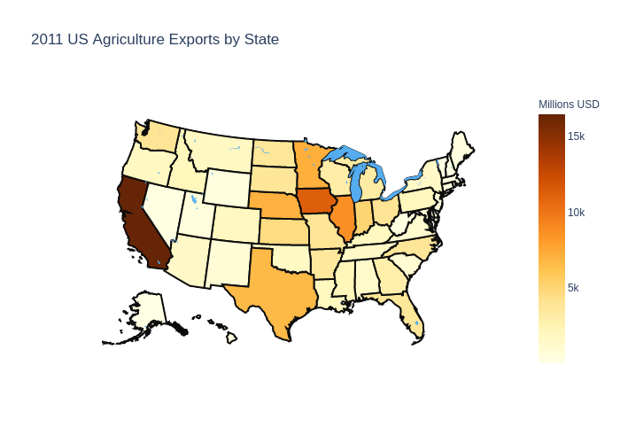
Real Data US Map Choropleth
1
2
df = pd.read_csv('2011_US_AGRI_Exports')
df.head()
| code | state | category | total exports | beef | pork | poultry | dairy | fruits fresh | fruits proc | total fruits | veggies fresh | veggies proc | total veggies | corn | wheat | cotton | text | |
|---|---|---|---|---|---|---|---|---|---|---|---|---|---|---|---|---|---|---|
| 0 | AL | Alabama | state | 1390.63 | 34.4 | 10.6 | 481.0 | 4.06 | 8.0 | 17.1 | 25.11 | 5.5 | 8.9 | 14.33 | 34.9 | 70.0 | 317.61 | Alabama<br>Beef 34.4 Dairy 4.06<br>Fruits 25.1... |
| 1 | AK | Alaska | state | 13.31 | 0.2 | 0.1 | 0.0 | 0.19 | 0.0 | 0.0 | 0.00 | 0.6 | 1.0 | 1.56 | 0.0 | 0.0 | 0.00 | Alaska<br>Beef 0.2 Dairy 0.19<br>Fruits 0.0 Ve... |
| 2 | AZ | Arizona | state | 1463.17 | 71.3 | 17.9 | 0.0 | 105.48 | 19.3 | 41.0 | 60.27 | 147.5 | 239.4 | 386.91 | 7.3 | 48.7 | 423.95 | Arizona<br>Beef 71.3 Dairy 105.48<br>Fruits 60... |
| 3 | AR | Arkansas | state | 3586.02 | 53.2 | 29.4 | 562.9 | 3.53 | 2.2 | 4.7 | 6.88 | 4.4 | 7.1 | 11.45 | 69.5 | 114.5 | 665.44 | Arkansas<br>Beef 53.2 Dairy 3.53<br>Fruits 6.8... |
| 4 | CA | California | state | 16472.88 | 228.7 | 11.1 | 225.4 | 929.95 | 2791.8 | 5944.6 | 8736.40 | 803.2 | 1303.5 | 2106.79 | 34.6 | 249.3 | 1064.95 | California<br>Beef 228.7 Dairy 929.95<br>Frui... |
1
2
3
4
5
6
7
8
9
10
11
12
13
14
15
16
17
18
19
20
21
22
23
data = dict(type='choropleth',
            colorscale = 'ylorbr',
            locations = df['code'],
            z = df['total exports'],
            locationmode = 'USA-states',
            text = df['text'],
            marker = dict(line = dict(color = 'rgb(12,12,12)',width = 2)),
            colorbar = {'title':"Millions USD"}
            )

layout = dict(title = '2011 US Agriculture Exports by State',
              geo = dict(showlakes = True,
                         lakecolor = 'rgb(85,173,240)')
             )

choromap = go.Figure(data = [data],layout = layout)
choromap = go.Figure(data = [data],layout = layout)
choromap.update_geos(
    visible=True,
    resolution=50,
    scope='usa',
    showcountries=True, countrycolor="Black",
    showsubunits=True, subunitcolor="Black")
1
2
3
# display static image
img_bytes = choromap.to_image(format="png")
Image(img_bytes)
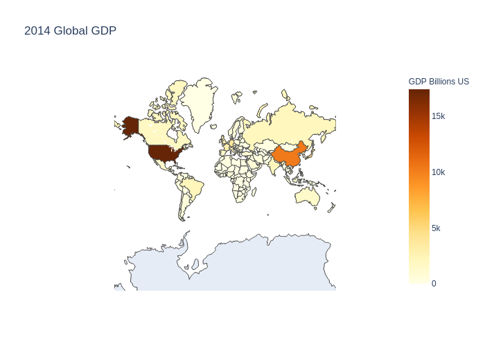
World GDP
1
2
df = pd.read_csv('2014_World_GDP')
df.head()
| COUNTRY | GDP (BILLIONS) | CODE | |
|---|---|---|---|
| 0 | Afghanistan | 21.71 | AFG |
| 1 | Albania | 13.40 | ALB |
| 2 | Algeria | 227.80 | DZA |
| 3 | American Samoa | 0.75 | ASM |
| 4 | Andorra | 4.80 | AND |
1
2
3
4
5
6
7
8
9
10
11
12
13
14
15
16
17
18
19
data = dict(
        type = 'choropleth',
        colorscale = 'ylorbr',
        locations = df['CODE'],
        z = df['GDP (BILLIONS)'],
        text = df['COUNTRY'],
        colorbar = {'title' : 'GDP Billions US'},
      )

layout = dict(
    title = '2014 Global GDP',
    geo = dict(
        showframe = False,
        projection = {'type':'mercator'}
    )
)

choromap = go.Figure(data = [data],layout = layout)
iplot(choromap)
1
2
3
# display static image
img_bytes = choromap.to_image(format="png")
Image(img_bytes)
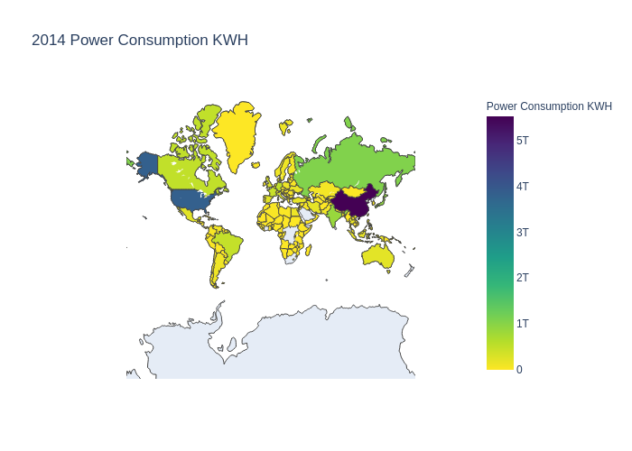
Word Power Consumption
1
2
df = pd.read_csv('2014_World_Power_Consumption')
df.head()
| Country | Power Consumption KWH | Text | |
|---|---|---|---|
| 0 | China | 5.523000e+12 | China 5,523,000,000,000 |
| 1 | United States | 3.832000e+12 | United 3,832,000,000,000 |
| 2 | European | 2.771000e+12 | European 2,771,000,000,000 |
| 3 | Russia | 1.065000e+12 | Russia 1,065,000,000,000 |
| 4 | Japan | 9.210000e+11 | Japan 921,000,000,000 |
1
2
3
4
5
6
7
8
9
10
11
12
13
14
15
16
17
18
19
data = dict(type = 'choropleth',
            colorscale = 'Viridis',
            reversescale = True,
            locations = df['Country'],
            locationmode = 'country names',  # l'incrocio della mappa si deve basare sul country names
            z = df['Power Consumption KWH'],
            text = df['Country'],
            colorbar = {'title' : 'Power Consumption KWH'},
           )

layout = dict(title = '2014 Power Consumption KWH',
              geo = dict(
                  showframe = False,
                  projection = {'type':'mercator'}
              )
             )

choromap = go.Figure(data = [data],layout = layout)
iplot(choromap,validate=False)
1
2
3
# display static image
img_bytes = choromap.to_image(format="png")
Image(img_bytes)
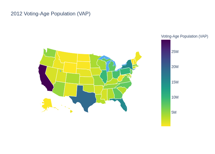
USA Choropleth
1
2
df = pd.read_csv('2012_Election_Data')
df.head()
| Year | ICPSR State Code | Alphanumeric State Code | State | VEP Total Ballots Counted | VEP Highest Office | VAP Highest Office | Total Ballots Counted | Highest Office | Voting-Eligible Population (VEP) | Voting-Age Population (VAP) | % Non-citizen | Prison | Probation | Parole | Total Ineligible Felon | State Abv | |
|---|---|---|---|---|---|---|---|---|---|---|---|---|---|---|---|---|---|
| 0 | 2012 | 41 | 1 | Alabama | NaN | 58.6% | 56.0% | NaN | 2,074,338 | 3,539,217 | 3707440.0 | 2.6% | 32,232 | 57,993 | 8,616 | 71,584 | AL |
| 1 | 2012 | 81 | 2 | Alaska | 58.9% | 58.7% | 55.3% | 301,694 | 300,495 | 511,792 | 543763.0 | 3.8% | 5,633 | 7,173 | 1,882 | 11,317 | AK |
| 2 | 2012 | 61 | 3 | Arizona | 53.0% | 52.6% | 46.5% | 2,323,579 | 2,306,559 | 4,387,900 | 4959270.0 | 9.9% | 35,188 | 72,452 | 7,460 | 81,048 | AZ |
| 3 | 2012 | 42 | 4 | Arkansas | 51.1% | 50.7% | 47.7% | 1,078,548 | 1,069,468 | 2,109,847 | 2242740.0 | 3.5% | 14,471 | 30,122 | 23,372 | 53,808 | AR |
| 4 | 2012 | 71 | 5 | California | 55.7% | 55.1% | 45.1% | 13,202,158 | 13,038,547 | 23,681,837 | 28913129.0 | 17.4% | 119,455 | 0 | 89,287 | 208,742 | CA |
1
2
3
4
5
6
7
8
9
10
11
12
13
14
15
16
17
18
19
20
21
data = dict(type = 'choropleth',
            colorscale = 'Viridis',
            reversescale = True,
            locations = df['State Abv'],
            locationmode = 'USA-states',
            z = df['Voting-Age Population (VAP)'],
            text = df['State'],
            marker = dict(line = dict(color = 'rgb(255,255,255)',width = 1)),
            colorbar = {'title' : 'Voting-Age Population (VAP)'}
           )

layout = dict(title = '2012 Voting-Age Population (VAP)',
              geo = dict(
                  scope = "usa",
                  showlakes = True,
                  lakecolor = 'rgb(85,173,240)'
                  )
             )

choromap = go.Figure(data = [data],layout = layout)
iplot(choromap,validate=False)
1
2
3
# display static image
img_bytes = choromap.to_image(format="png")
Image(img_bytes)