Utilizzo l’environment conda py3
SVM
Prima o poi pubblico gli appunti di università!

I kernel permettono di fare trasformazioni ai dati e quindi di separare casi non linearmente separabili.
1
2
3
4
5
6
7
8
9
10
11
12
| # lib
import pandas as pd
import numpy as np
import matplotlib.pyplot as plt
import seaborn as sns
%matplotlib inline
from sklearn.datasets import load_breast_cancer
from sklearn.model_selection import train_test_split
from sklearn.svm import SVC
from sklearn.metrics import classification_report,confusion_matrix
from sklearn.model_selection import GridSearchCV
|
1
2
3
| # cancer Bunch
cancer = load_breast_cancer()
cancer.keys()
|
1
| dict_keys(['data', 'target', 'frame', 'target_names', 'DESCR', 'feature_names', 'filename'])
|
1
2
| # description of the Bunch
print(cancer['DESCR'])
|
1
2
3
4
5
6
7
8
9
10
11
12
13
14
15
16
17
18
19
20
21
22
23
24
25
26
27
28
29
30
31
32
33
| .. _breast_cancer_dataset:
Breast cancer wisconsin (diagnostic) dataset
--------------------------------------------
**Data Set Characteristics:**
:Number of Instances: 569
:Number of Attributes: 30 numeric, predictive attributes and the class
:Attribute Information:
- radius (mean of distances from center to points on the perimeter)
- texture (standard deviation of gray-scale values)
- perimeter
- area
- smoothness (local variation in radius lengths)
- compactness (perimeter^2 / area - 1.0)
- concavity (severity of concave portions of the contour)
- concave points (number of concave portions of the contour)
- symmetry
- fractal dimension ("coastline approximation" - 1)
The mean, standard error, and "worst" or largest (mean of the three
worst/largest values) of these features were computed for each image,
resulting in 30 features. For instance, field 0 is Mean Radius, field
10 is Radius SE, field 20 is Worst Radius.
- class:
- WDBC-Malignant
- WDBC-Benign
...
|
1
2
| # columns
cancer['feature_names']
|
1
2
3
4
5
6
7
8
9
10
| array(['mean radius', 'mean texture', 'mean perimeter', 'mean area',
'mean smoothness', 'mean compactness', 'mean concavity',
'mean concave points', 'mean symmetry', 'mean fractal dimension',
'radius error', 'texture error', 'perimeter error', 'area error',
'smoothness error', 'compactness error', 'concavity error',
'concave points error', 'symmetry error',
'fractal dimension error', 'worst radius', 'worst texture',
'worst perimeter', 'worst area', 'worst smoothness',
'worst compactness', 'worst concavity', 'worst concave points',
'worst symmetry', 'worst fractal dimension'], dtype='<U23')
|
1
2
3
| # dataframe (solo le esplicative)
df_feat = pd.DataFrame(cancer['data'],columns=cancer['feature_names'])
df_feat.info()
|
1
2
3
4
5
6
7
8
9
10
11
12
| <class 'pandas.core.frame.DataFrame'>
RangeIndex: 569 entries, 0 to 568
Data columns (total 30 columns):
# Column Non-Null Count Dtype
--- ------ -------------- -----
0 mean radius 569 non-null float64
1 mean texture 569 non-null float64
....................................................
28 worst symmetry 569 non-null float64
29 worst fractal dimension 569 non-null float64
dtypes: float64(30)
memory usage: 133.5 KB
|
1
2
3
| # dataframe (target)
df_target = pd.DataFrame(cancer['target'],columns=['Cancer'])
df_target['Cancer'].value_counts()
|
1
2
3
| 1 357
0 212
Name: Cancer, dtype: int64
|
EDA
skipped today :))
SVM Model
1
2
3
4
5
| # train test set
X = df_feat
y = cancer['target'] # oppure np.ravel(df_target) per renderlo array
X_train, X_test, y_train, y_test = train_test_split(X,y,test_size=0.30, random_state=101)
|
1
2
3
| # svm
model = SVC()
model.fit(X_train,y_train)
|
1
2
| # predictions
predictions = model.predict(X_test)
|
1
2
3
4
5
| # metrics
print('\nConfusion Matrix:')
print(confusion_matrix(y_test,predictions))
print('\nClassification metrics:')
print(classification_report(y_test,predictions))
|
1
2
3
4
5
6
7
8
9
10
11
12
13
| Confusion Matrix:
[[ 56 10]
[ 3 102]]
Classification metrics:
precision recall f1-score support
0 0.95 0.85 0.90 66
1 0.91 0.97 0.94 105
accuracy 0.92 171
macro avg 0.93 0.91 0.92 171
weighted avg 0.93 0.92 0.92 171
|
GridSearch
1
2
3
4
5
| # grid
param_grid = {'C': [0.01,0.1,1, 10, 100, 1000], 'gamma': [1,0.1,0.01,0.001,0.0001,0.00001], 'kernel': ['rbf']}
# large C low bias high variance e viceversa per C elevato
grid = GridSearchCV(SVC(),param_grid,refit=True,verbose=3)
# verbose più è alto e più lascia traccia
|
1
2
| # grid fitting
grid.fit(X_train,y_train)
|
1
2
3
4
5
6
7
8
9
10
11
12
13
14
15
16
| Fitting 5 folds for each of 36 candidates, totalling 180 fits
[CV] C=0.01, gamma=1, kernel=rbf .....................................
[CV] ......... C=0.01, gamma=1, kernel=rbf, score=0.637, total= 0.0s
...
[CV] C=1000, gamma=1e-05, kernel=rbf .................................
[CV] ..... C=1000, gamma=1e-05, kernel=rbf, score=0.975, total= 0.0s
[Parallel(n_jobs=1)]: Done 180 out of 180 | elapsed: 2.3s finished
GridSearchCV(estimator=SVC(),
param_grid={'C': [0.01, 0.1, 1, 10, 100, 1000],
'gamma': [1, 0.1, 0.01, 0.001, 0.0001, 1e-05],
'kernel': ['rbf']},
verbose=3)
|
1
2
| # best parameters
grid.best_params_
|
1
| {'C': 100, 'gamma': 1e-05, 'kernel': 'rbf'}
|
1
2
| # best estimators
grid.best_estimator_
|
1
| SVC(C=100, gamma=1e-05)
|
1
2
| # predictions
predictions_grid = grid.predict(X_test)
|
1
2
3
4
5
| # metrics
print('\nConfusion Matrix:')
print(confusion_matrix(y_test,predictions_grid))
print('\nClassification metrics:')
print(classification_report(y_test,predictions_grid))
|
1
2
3
4
5
6
7
8
9
10
11
12
13
| Confusion Matrix:
[[ 59 7]
[ 4 101]]
Classification metrics:
precision recall f1-score support
0 0.94 0.89 0.91 66
1 0.94 0.96 0.95 105
accuracy 0.94 171
macro avg 0.94 0.93 0.93 171
weighted avg 0.94 0.94 0.94 171
|
1
2
| # pulisco il workspace
%reset -f
|
Iris Dataset
The famous Iris flower data set.
The Iris flower data set or Fisher’s Iris data set is a multivariate data set introduced by Sir Ronald Fisher in the 1936 as an example of discriminant analysis.
The data set consists of 50 samples from each of three species of Iris (Iris setosa, Iris virginica and Iris versicolor), so 150 total samples. Four features were measured from each sample: the length and the width of the sepals and petals, in centimeters.
Here’s a picture of the three different Iris types:
1
2
3
4
| # The Iris Setosa
from IPython.display import Image
url = 'http://upload.wikimedia.org/wikipedia/commons/5/56/Kosaciec_szczecinkowaty_Iris_setosa.jpg'
Image(url,width=300, height=300)
|

1
2
3
4
| # The Iris Versicolor
from IPython.display import Image
url = 'http://upload.wikimedia.org/wikipedia/commons/4/41/Iris_versicolor_3.jpg'
Image(url,width=300, height=300)
|

1
2
3
4
| # The Iris Virginica
from IPython.display import Image
url = 'http://upload.wikimedia.org/wikipedia/commons/9/9f/Iris_virginica.jpg'
Image(url,width=300, height=300)
|

The iris dataset contains measurements for 150 iris flowers from three different species.
The three classes in the Iris dataset:
1
2
3
| Iris-setosa (n=50)
Iris-versicolor (n=50)
Iris-virginica (n=50)
|
The four features of the Iris dataset:
1
2
3
4
| sepal length in cm
sepal width in cm
petal length in cm
petal width in cm
|
1
2
3
4
5
6
7
8
9
10
11
12
| # lib
import pandas as pd
import numpy as np
import matplotlib.pyplot as plt
import seaborn as sns
%matplotlib inline
from sklearn.datasets import load_breast_cancer
from sklearn.model_selection import train_test_split
from sklearn.svm import SVC
from sklearn.metrics import classification_report,confusion_matrix
from sklearn.model_selection import GridSearchCV
|
1
2
3
| # df
iris = sns.load_dataset('iris')
iris.head()
|
|
sepal_length |
sepal_width |
petal_length |
petal_width |
species |
| 0 |
5.1 |
3.5 |
1.4 |
0.2 |
setosa |
| 1 |
4.9 |
3.0 |
1.4 |
0.2 |
setosa |
| 2 |
4.7 |
3.2 |
1.3 |
0.2 |
setosa |
| 3 |
4.6 |
3.1 |
1.5 |
0.2 |
setosa |
| 4 |
5.0 |
3.6 |
1.4 |
0.2 |
setosa |
EDA
1
2
3
4
5
6
7
8
9
10
11
12
| <class 'pandas.core.frame.DataFrame'>
RangeIndex: 150 entries, 0 to 149
Data columns (total 5 columns):
# Column Non-Null Count Dtype
--- ------ -------------- -----
0 sepal_length 150 non-null float64
1 sepal_width 150 non-null float64
2 petal_length 150 non-null float64
3 petal_width 150 non-null float64
4 species 150 non-null object
dtypes: float64(4), object(1)
memory usage: 6.0+ KB
|
|
sepal_length |
sepal_width |
petal_length |
petal_width |
| count |
150.000000 |
150.000000 |
150.000000 |
150.000000 |
| mean |
5.843333 |
3.057333 |
3.758000 |
1.199333 |
| std |
0.828066 |
0.435866 |
1.765298 |
0.762238 |
| min |
4.300000 |
2.000000 |
1.000000 |
0.100000 |
| 25% |
5.100000 |
2.800000 |
1.600000 |
0.300000 |
| 50% |
5.800000 |
3.000000 |
4.350000 |
1.300000 |
| 75% |
6.400000 |
3.300000 |
5.100000 |
1.800000 |
| max |
7.900000 |
4.400000 |
6.900000 |
2.500000 |
1
2
3
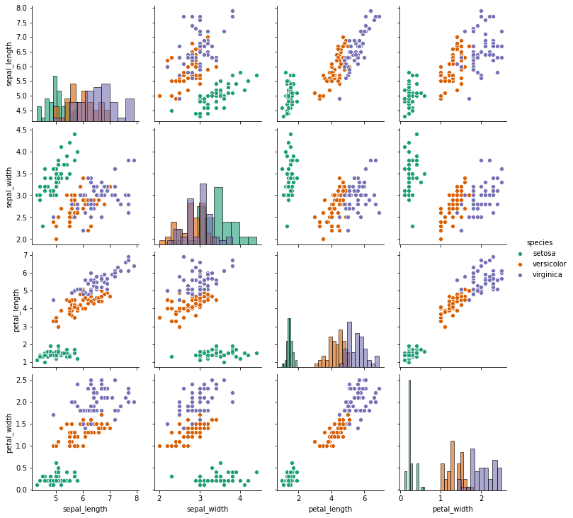
| # pairplot
sns.pairplot(iris,hue='species',diag_kind='hist',diag_kws=dict(edgecolor='black',alpha=0.6),palette='Dark2')
# setosa sembra più separabile
|
1
| <seaborn.axisgrid.PairGrid at 0x7f2cb4206390>
|
1
2
3
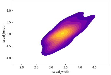
| # kde plot per 'setosa'
setosa = iris[iris['species']=='setosa']
sns.kdeplot(setosa['sepal_width'],setosa['sepal_length'],cmap="plasma",shade=True,shade_lowest=False)
|
1
| <matplotlib.axes._subplots.AxesSubplot at 0x7f2cb4363f50>
|
Model
1
2
3
4
| # train test set
X = iris.drop('species',axis=1)
y = iris['species']
X_train, X_test, y_train, y_test = train_test_split(X,y,test_size=0.30, random_state=101)
|
1
2
3
4
5
6
7
8
9
10
11
12
| # svm
model = SVC()
model.fit(X_train,y_train)
# predictions
predictions = model.predict(X_test)
# metrics
print('\nConfusion Matrix:')
print(confusion_matrix(y_test,predictions))
print('\nClassification metrics:')
print(classification_report(y_test,predictions))
|
1
2
3
4
5
6
7
8
9
10
11
12
13
14
15
| Confusion Matrix:
[[13 0 0]
[ 0 19 1]
[ 0 0 12]]
Classification metrics:
precision recall f1-score support
setosa 1.00 1.00 1.00 13
versicolor 1.00 0.95 0.97 20
virginica 0.92 1.00 0.96 12
accuracy 0.98 45
macro avg 0.97 0.98 0.98 45
weighted avg 0.98 0.98 0.98 45
|
1
2
| # pulisco il workspace
%reset -f
|