Python: K Means Clustering
Utilizzo l’environment conda py3
1
~$ conda activate py3
K Means Clustering
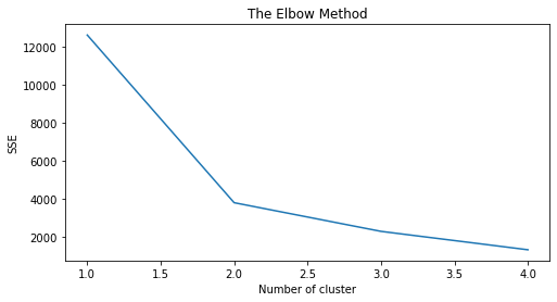
Cercare un numero k di cluster affiché il k-esimo sia quello a far cadere bruscamente il valore di SSE (Sum of Squared Error) – Elbow method
1
2
3
4
5
6
7
8
import pandas as pd
import numpy as np
import seaborn as sns
import matplotlib.pyplot as plt
%matplotlib inline

from sklearn.datasets import make_blobs
from sklearn.cluster import KMeans
1
2
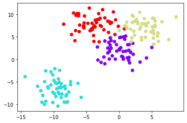
# Create random data
data = make_blobs(n_samples=200, n_features=2, centers=4, cluster_std=1.8,random_state=101)
1
type(data)
1
tuple
1
data[0].shape
1
(200, 2)
1
2
# plot
plt.scatter(data[0][:,0],data[0][:,1],c=data[1],cmap='rainbow')
1
<matplotlib.collections.PathCollection at 0x7f2ca62dda90>
1
2
3
# cluster k Means
kmeans = KMeans(n_clusters=4)
kmeans.fit(data[0])
1
KMeans(n_clusters=4)
1
2
# centroidi
kmeans.cluster_centers_
1
2
3
4
array([[-4.13591321,  7.95389851],
       [-9.46941837, -6.56081545],
       [ 3.71749226,  7.01388735],
       [-0.0123077 ,  2.13407664]])
Supervised metrics
1
2
3
# label sono i predetti e data[1] sono gli osservati
print(kmeans.labels_.shape)
print(data[1].shape)
1
2
(200,)
(200,)
1
2
3
4
5
6
7
8
9
10
11
12
13
14
15
16
# vediamo come si comporta la matrice di confusione (nb. il metodo è non supervisionato ed è solo una verifica)
from sklearn.metrics import classification_report,confusion_matrix

# il cluster non conoscendo l'ordine confonde la terza classe con la quarta (index 2 e 3)
# costruisco funzione per invertire (il 100000 mi serve come valore temporaneo per lo switch)
def inverti(x, questo, questaltro):
    uno = np.where(x==questo, 100000, x)
    due = np.where(uno==questaltro, questo, uno)
    tre = np.where(due==100000,questaltro,due)
    return(tre)

# metrics
print('\nConfusion Matrix:')
print(confusion_matrix(data[1],inverti(kmeans.labels_,2,3)))
print('\nClassification metrics:')
print(classification_report(data[1],inverti(kmeans.labels_,2,3)))
1
2
3
4
5
6
7
8
9
10
11
12
13
14
15
16
17
Confusion Matrix:
[[49  0  1  0]
 [ 0 50  0  0]
 [ 3  0 47  0]
 [ 2  0  2 46]]

Classification metrics:
              precision    recall  f1-score   support

           0       0.91      0.98      0.94        50
           1       1.00      1.00      1.00        50
           2       0.94      0.94      0.94        50
           3       1.00      0.92      0.96        50

    accuracy                           0.96       200
   macro avg       0.96      0.96      0.96       200
weighted avg       0.96      0.96      0.96       200
1
2
3
4
5
6
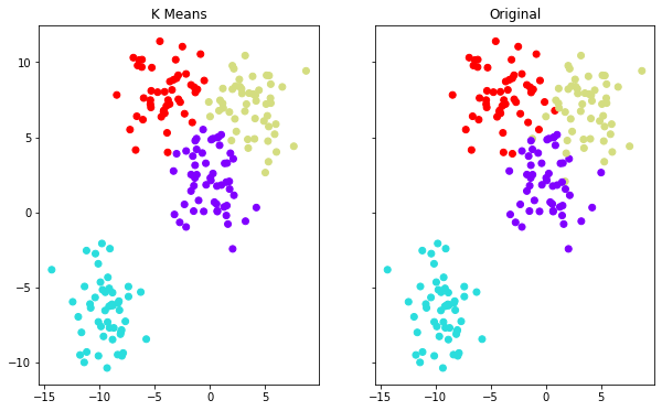
# plot confronto (separati)
f, (ax1, ax2) = plt.subplots(1, 2, sharey=True,figsize=(10,6))
ax1.set_title('K Means')
ax1.scatter(data[0][:,0],data[0][:,1],c=inverti(kmeans.labels_,2,3),cmap='rainbow')
ax2.set_title("Original")
ax2.scatter(data[0][:,0],data[0][:,1],c=data[1],cmap='rainbow')
1
<matplotlib.collections.PathCollection at 0x7f2ca58edb90>
1
2
3
4
5
6
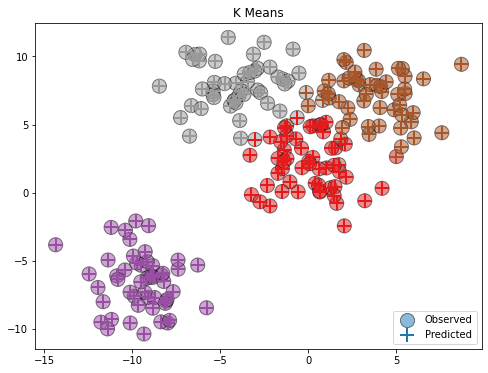
# plot confronto (uniti)
plt.figure(figsize=(8,6))
plt.scatter(data[0][:,0],data[0][:,1],c=data[1],cmap='Set1',marker='o',alpha=0.5,s=200,edgecolors='black',label='Observed')
plt.scatter(data[0][:,0],data[0][:,1],c=inverti(kmeans.labels_,2,3),cmap='Set1',marker='+',s=200,linewidth=2,label='Predicted')
plt.legend(loc='lower right')
plt.title('K Means')
1
Text(0.5, 1.0, 'K Means')
Elbow Method
Il Silhouette Coefficient più è alto meglio è
1
from sklearn.metrics import silhouette_score
1
2
3
4
5
6
7
8
9
# Fit KMeans and calculate SSE for each k
sse = {}
for k in range(1, 5):
    kmeans = KMeans(n_clusters=k, max_iter=1000, random_state=1).fit(data[0])
    sse[k] = kmeans.inertia_ # Inertia: Sum of distances of samples to their closest cluster center
    label = kmeans.labels_
    if k == 1: continue
    sil_coeff = silhouette_score(data[0], label, metric='euclidean')
    print("For n_clusters={}, The Silhouette Coefficient is {}".format(k, sil_coeff))
1
2
3
For n_clusters=2, The Silhouette Coefficient is 0.6490840372235874
For n_clusters=3, The Silhouette Coefficient is 0.5021702155773816
For n_clusters=4, The Silhouette Coefficient is 0.5519773421333025
1
2
3
4
5
6
# Elbow Method
plt.figure(figsize=(8,4))
plt.title('The Elbow Method')
plt.xlabel('Number of cluster')
plt.ylabel('SSE')
sns.lineplot(x=list(sse.keys()), y=list(sse.values()))
1
<matplotlib.axes._subplots.AxesSubplot at 0x7f2ca5711e50>