
Python: Principal Component Analysis
Utilizzo l’environment conda py3
1
~$ conda activate py3
PCA


1
2
3
4
5
6
7
8
9
10
# lib
import matplotlib.pyplot as plt
import pandas as pd
import numpy as np
import seaborn as sns
%matplotlib inline

from sklearn.datasets import load_breast_cancer
from sklearn.preprocessing import StandardScaler
from sklearn.decomposition import PCA
1
2
3
# cancer data
cancer = load_breast_cancer()
cancer.keys()
1
dict_keys(['data', 'target', 'frame', 'target_names', 'DESCR', 'feature_names', 'filename'])
1
2
3
# df
df = pd.DataFrame(cancer['data'],columns=cancer['feature_names'])
df.head()
| mean radius | mean texture | mean perimeter | mean area | mean smoothness | mean compactness | mean concavity | mean concave points | mean symmetry | mean fractal dimension | ... | worst radius | worst texture | worst perimeter | worst area | worst smoothness | worst compactness | worst concavity | worst concave points | worst symmetry | worst fractal dimension | |
|---|---|---|---|---|---|---|---|---|---|---|---|---|---|---|---|---|---|---|---|---|---|
| 0 | 17.99 | 10.38 | 122.80 | 1001.0 | 0.11840 | 0.27760 | 0.3001 | 0.14710 | 0.2419 | 0.07871 | ... | 25.38 | 17.33 | 184.60 | 2019.0 | 0.1622 | 0.6656 | 0.7119 | 0.2654 | 0.4601 | 0.11890 |
| 1 | 20.57 | 17.77 | 132.90 | 1326.0 | 0.08474 | 0.07864 | 0.0869 | 0.07017 | 0.1812 | 0.05667 | ... | 24.99 | 23.41 | 158.80 | 1956.0 | 0.1238 | 0.1866 | 0.2416 | 0.1860 | 0.2750 | 0.08902 |
| 2 | 19.69 | 21.25 | 130.00 | 1203.0 | 0.10960 | 0.15990 | 0.1974 | 0.12790 | 0.2069 | 0.05999 | ... | 23.57 | 25.53 | 152.50 | 1709.0 | 0.1444 | 0.4245 | 0.4504 | 0.2430 | 0.3613 | 0.08758 |
| 3 | 11.42 | 20.38 | 77.58 | 386.1 | 0.14250 | 0.28390 | 0.2414 | 0.10520 | 0.2597 | 0.09744 | ... | 14.91 | 26.50 | 98.87 | 567.7 | 0.2098 | 0.8663 | 0.6869 | 0.2575 | 0.6638 | 0.17300 |
| 4 | 20.29 | 14.34 | 135.10 | 1297.0 | 0.10030 | 0.13280 | 0.1980 | 0.10430 | 0.1809 | 0.05883 | ... | 22.54 | 16.67 | 152.20 | 1575.0 | 0.1374 | 0.2050 | 0.4000 | 0.1625 | 0.2364 | 0.07678 |
5 rows × 30 columns
1
2
3
4
# scaling data
scaler = StandardScaler()
scaler.fit(df)
scaled_data = scaler.transform(df)
1
2
3
# PCA
pca = PCA(n_components=2)
pca.fit(scaled_data)
1
PCA(n_components=2)
1
2
# trasform data to two components (da 30 colonne a 2)
x_pca = pca.transform(scaled_data)
1
2
print(scaled_data.shape)
print(x_pca.shape)
1
2
(569, 30)
(569, 2)
1
2
3
4
5
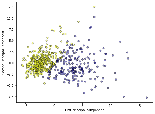
# plot PCA
plt.figure(figsize=(8,6))
plt.scatter(x_pca[:,0],x_pca[:,1],c=cancer['target'],cmap='plasma',edgecolors='black',alpha=0.5)
plt.xlabel('First principal component')
plt.ylabel('Second Principal Component')
1
Text(0, 0.5, 'Second Principal Component')
Coefficients
1
2
3
4
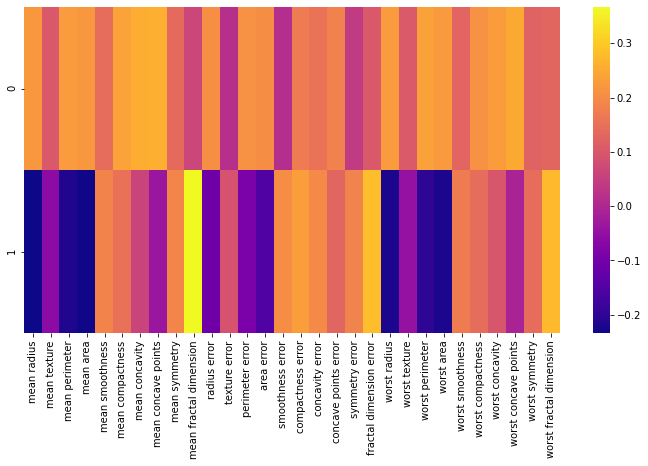
# interpretazioni coefficienti
# correlazione tra le variabili e le componenti
df_comp = pd.DataFrame(pca.components_,columns=cancer['feature_names'])
df_comp.head()
| mean radius | mean texture | mean perimeter | mean area | mean smoothness | mean compactness | mean concavity | mean concave points | mean symmetry | mean fractal dimension | ... | worst radius | worst texture | worst perimeter | worst area | worst smoothness | worst compactness | worst concavity | worst concave points | worst symmetry | worst fractal dimension | |
|---|---|---|---|---|---|---|---|---|---|---|---|---|---|---|---|---|---|---|---|---|---|
| 0 | 0.218902 | 0.103725 | 0.227537 | 0.220995 | 0.142590 | 0.239285 | 0.258400 | 0.260854 | 0.138167 | 0.064363 | ... | 0.227997 | 0.104469 | 0.236640 | 0.224871 | 0.127953 | 0.210096 | 0.228768 | 0.250886 | 0.122905 | 0.131784 |
| 1 | -0.233857 | -0.059706 | -0.215181 | -0.231077 | 0.186113 | 0.151892 | 0.060165 | -0.034768 | 0.190349 | 0.366575 | ... | -0.219866 | -0.045467 | -0.199878 | -0.219352 | 0.172304 | 0.143593 | 0.097964 | -0.008257 | 0.141883 | 0.275339 |
2 rows × 30 columns
1
2
3
# heatmap
plt.figure(figsize=(12,6))
sns.heatmap(df_comp,cmap='plasma')
1
<matplotlib.axes._subplots.AxesSubplot at 0x7fee706d6d50>
Biplot
1
2
3
4
5
6
7
8
9
10
11
12
13
14
15
16
17
18
19
20
21
22
23
24
25
26
27
28
29
30
31
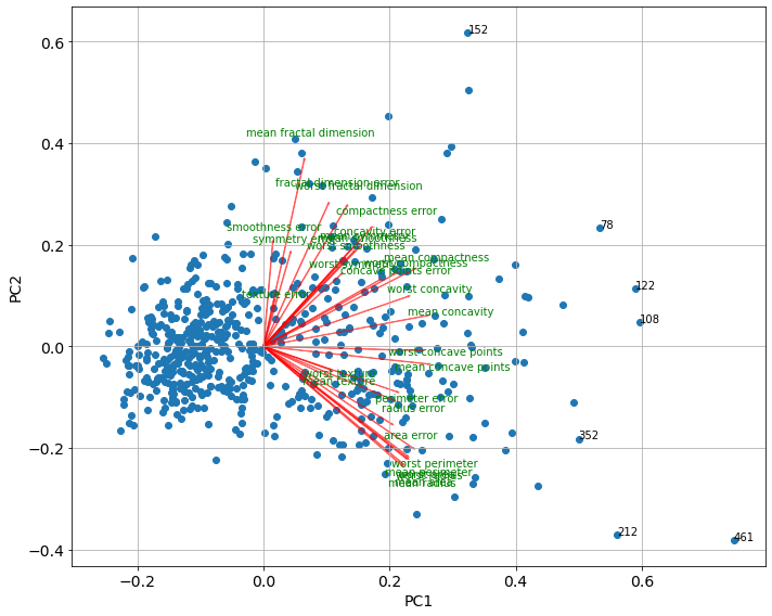
# il biplot è la rappresentazione grafica delle due prime componenti
# utile anche per identificare gli outliers
# funzione per il biplot
def biplot(score,coeff,y=None,labels=None):
xs = score[:,0] # projection of PC1
ys = score[:,1] # projection of PC2
n = coeff.shape[0]
scalex = 1.0/(xs.max() - xs.min())
scaley = 1.0/(ys.max() - ys.min())
plt.scatter(xs * scalex,ys * scaley, c = y)
# aggiungo frecce
for i in range(n):
plt.arrow(0, 0, coeff[i,0], coeff[i,1],color = 'r',alpha = 0.5)
if labels is None:
plt.text(coeff[i,0]* 1.15, coeff[i,1] * 1.15, "Var"+str(i+1), color = 'g', ha = 'center', va = 'center')
else:
plt.text(coeff[i,0]* 1.15, coeff[i,1] * 1.15, labels[i], color = 'g', ha = 'center', va = 'center')
# aggiungo flag outliers
for i in range(len(xs)):
if ((xs[i]>np.quantile(xs,0.99)) | (ys[i]>np.quantile(xs,0.99))):
plt.text(xs[i] * scalex,ys[i] * scaley, str(i))
# etichette
plt.xlabel("PC{}".format(1), size=14)
plt.ylabel("PC{}".format(2), size=14)
plt.grid()
plt.tick_params(axis='both', which='both', labelsize=14)
plt.tight_layout()
1
2
3
4
5
6
7
8
# plot
plt.figure(figsize=(10,8))
biplot(score=x_pca,coeff=np.transpose(pca.components_),labels=df.columns)

# se ci fossero più componenti plotto solo le prime due (nb. sono array non dataframes)
# score=x_pca[:,0:2],coef=np.transpose(pca.components_[0:2, :])

# le variabili nella stessa direzione sono correlate
1
2
# esempio stessa direzione
np.corrcoef(df['worst perimeter'],df['mean perimeter'])[1,0]
1
0.9703868870426392
Outliers
1
2
3
# l'osservazione 461 è outliers per la prima componente, che ha coefficienti positivi verso le variabili
# infatti i valori delle sue variabili sono vicini ai massimi (vedi il describe)
x_pca[461,]
1
array([16.31923323, -7.7758528 ])
1
2
3
4
# l'osservazione 152 è outliers per la seconda componente
# la PC2 ha coefficienti negativi verso le variabili tranne per 'mean fractal dimension'
# infatti i valori delle sue variabili sono vicini ai minimi, tranne per 'mean fractal dimension' che è elevata
x_pca[152,]
1
array([ 7.09330671, 12.57319423])
1
2
# describe stats assieme a due outliers
pd.concat([df.describe(),df.iloc[[461,152]]],axis=0)
| mean radius | mean texture | mean perimeter | mean area | mean smoothness | mean compactness | mean concavity | mean concave points | mean symmetry | mean fractal dimension | ... | worst radius | worst texture | worst perimeter | worst area | worst smoothness | worst compactness | worst concavity | worst concave points | worst symmetry | worst fractal dimension | |
|---|---|---|---|---|---|---|---|---|---|---|---|---|---|---|---|---|---|---|---|---|---|
| count | 569.000000 | 569.000000 | 569.000000 | 569.000000 | 569.000000 | 569.000000 | 569.000000 | 569.000000 | 569.000000 | 569.000000 | ... | 569.000000 | 569.000000 | 569.000000 | 569.000000 | 569.000000 | 569.000000 | 569.000000 | 569.000000 | 569.000000 | 569.000000 |
| mean | 14.127292 | 19.289649 | 91.969033 | 654.889104 | 0.096360 | 0.104341 | 0.088799 | 0.048919 | 0.181162 | 0.062798 | ... | 16.269190 | 25.677223 | 107.261213 | 880.583128 | 0.132369 | 0.254265 | 0.272188 | 0.114606 | 0.290076 | 0.083946 |
| std | 3.524049 | 4.301036 | 24.298981 | 351.914129 | 0.014064 | 0.052813 | 0.079720 | 0.038803 | 0.027414 | 0.007060 | ... | 4.833242 | 6.146258 | 33.602542 | 569.356993 | 0.022832 | 0.157336 | 0.208624 | 0.065732 | 0.061867 | 0.018061 |
| min | 6.981000 | 9.710000 | 43.790000 | 143.500000 | 0.052630 | 0.019380 | 0.000000 | 0.000000 | 0.106000 | 0.049960 | ... | 7.930000 | 12.020000 | 50.410000 | 185.200000 | 0.071170 | 0.027290 | 0.000000 | 0.000000 | 0.156500 | 0.055040 |
| 25% | 11.700000 | 16.170000 | 75.170000 | 420.300000 | 0.086370 | 0.064920 | 0.029560 | 0.020310 | 0.161900 | 0.057700 | ... | 13.010000 | 21.080000 | 84.110000 | 515.300000 | 0.116600 | 0.147200 | 0.114500 | 0.064930 | 0.250400 | 0.071460 |
| 50% | 13.370000 | 18.840000 | 86.240000 | 551.100000 | 0.095870 | 0.092630 | 0.061540 | 0.033500 | 0.179200 | 0.061540 | ... | 14.970000 | 25.410000 | 97.660000 | 686.500000 | 0.131300 | 0.211900 | 0.226700 | 0.099930 | 0.282200 | 0.080040 |
| 75% | 15.780000 | 21.800000 | 104.100000 | 782.700000 | 0.105300 | 0.130400 | 0.130700 | 0.074000 | 0.195700 | 0.066120 | ... | 18.790000 | 29.720000 | 125.400000 | 1084.000000 | 0.146000 | 0.339100 | 0.382900 | 0.161400 | 0.317900 | 0.092080 |
| max | 28.110000 | 39.280000 | 188.500000 | 2501.000000 | 0.163400 | 0.345400 | 0.426800 | 0.201200 | 0.304000 | 0.097440 | ... | 36.040000 | 49.540000 | 251.200000 | 4254.000000 | 0.222600 | 1.058000 | 1.252000 | 0.291000 | 0.663800 | 0.207500 |
| 461 | 27.420000 | 26.270000 | 186.900000 | 2501.000000 | 0.108400 | 0.198800 | 0.363500 | 0.168900 | 0.206100 | 0.056230 | ... | 36.040000 | 31.370000 | 251.200000 | 4254.000000 | 0.135700 | 0.425600 | 0.683300 | 0.262500 | 0.264100 | 0.074270 |
| 152 | 9.731000 | 15.340000 | 63.780000 | 300.200000 | 0.107200 | 0.159900 | 0.410800 | 0.078570 | 0.254800 | 0.092960 | ... | 11.020000 | 19.490000 | 71.040000 | 380.500000 | 0.129200 | 0.277200 | 0.821600 | 0.157100 | 0.310800 | 0.125900 |
10 rows × 30 columns
1
2
# pulisco il workspace
%reset -f