
Python: Recommender system
Utilizzo l’environment conda py3
1
~$ conda activate py3
Indice
- Recommender system
- Recommending Similar Movies by Correlations
- Collaborative Filtering
- Memory-Based Collaborative Filtering
- Model-Based Collaborative Filtering
- More resources
Recommender system
Collaborative Filtering (CF) in funzione della conoscenza della rete sociale
- Memory-Based CF (eg. Cosine Similarity)
- Model-Based CF (eg. Singular Value Decomposition)
Content-Based in funzione della similarità dei metadati degli item
1
2
3
4
5
6
7
8
9
10
11
12
13
14
15
16
17
18
19
# lib
import numpy as np
import pandas as pd
from datetime import datetime

# per mostrare le stringhe al completo
pd.set_option('display.max_colwidth', None)

import matplotlib.pyplot as plt
import seaborn as sns
sns.set_style('white')
%matplotlib inline

from sklearn.model_selection import train_test_split
from sklearn.metrics.pairwise import pairwise_distances
from sklearn.metrics import mean_squared_error
from math import sqrt
import scipy.sparse as sp
from scipy.sparse.linalg import svds
1
2
3
4
# df users
column_names = ['user_id', 'item_id', 'rating', 'timestamp']
df = pd.read_csv('u.data', sep='\t', names=column_names)
df.head()
| user_id | item_id | rating | timestamp | |
|---|---|---|---|---|
| 0 | 0 | 50 | 5 | 881250949 |
| 1 | 0 | 172 | 5 | 881250949 |
| 2 | 0 | 133 | 1 | 881250949 |
| 3 | 196 | 242 | 3 | 881250949 |
| 4 | 186 | 302 | 3 | 891717742 |
1
2
3
# creo colonna data da timeStamp
df['user_Date'] = pd.to_datetime(df['timestamp'].apply(lambda x: pd.Timestamp(x, unit='s')))
df['user_Year'] = df['user_Date'].apply(lambda x: x.year)
1
df.head()
| user_id | item_id | rating | timestamp | user_Date | user_Year | |
|---|---|---|---|---|---|---|
| 0 | 0 | 50 | 5 | 881250949 | 1997-12-04 15:55:49 | 1997 |
| 1 | 0 | 172 | 5 | 881250949 | 1997-12-04 15:55:49 | 1997 |
| 2 | 0 | 133 | 1 | 881250949 | 1997-12-04 15:55:49 | 1997 |
| 3 | 196 | 242 | 3 | 881250949 | 1997-12-04 15:55:49 | 1997 |
| 4 | 186 | 302 | 3 | 891717742 | 1998-04-04 19:22:22 | 1998 |
1
2
3
# df movies
movie_titles = pd.read_csv("Movie_Id_Titles")
movie_titles.head()
| item_id | title | |
|---|---|---|
| 0 | 1 | Toy Story (1995) |
| 1 | 2 | GoldenEye (1995) |
| 2 | 3 | Four Rooms (1995) |
| 3 | 4 | Get Shorty (1995) |
| 4 | 5 | Copycat (1995) |
1
movie_titles.info()
1
2
3
4
5
6
7
8
9
<class 'pandas.core.frame.DataFrame'>
RangeIndex: 1682 entries, 0 to 1681
Data columns (total 2 columns):
 #   Column   Non-Null Count  Dtype
---  ------   --------------  -----
 0   item_id  1682 non-null   int64
 1   title    1682 non-null   object
dtypes: int64(1), object(1)
memory usage: 26.4+ KB
1
2
3
# estraggo la data dal titolo (esercizio personale)
# l'espressione seguente è limitata ma può tornarmi utile in futuro, ci sono diversi casi che non riesce a gestire
# movie_titles['title'].str.split('(').apply(lambda x: x[1] if len(x) > 1 else 0)
1
2
# problema 1: alcuni non hanno le parentesi
movie_titles[~movie_titles['title'].astype(str).str.contains('\(')]
| item_id | title | |
|---|---|---|
| 266 | 267 | unknown |
1
2
# problema 2: la data non è sempre la prima parentesi (risolvibile con x[-1])
movie_titles[movie_titles['title']=='Scream of Stone (Schrei aus Stein) (1991)']
| item_id | title | |
|---|---|---|
| 1681 | 1682 | Scream of Stone (Schrei aus Stein) (1991) |
1
2
# problema 3: la data non è sempre l'ultima parentesi (solo un caso, potenzialmente risolvibile a mano)
movie_titles[movie_titles['title']=='Land Before Time III: The Time of the Great Giving (1995) (V)']
| item_id | title | |
|---|---|---|
| 1411 | 1412 | Land Before Time III: The Time of the Great Giving (1995) (V) |
1
2
# problema 4: dopo la data ci può essere uno spazio (risolvibile con .strip)
movie_titles[movie_titles['title']=='Marlene Dietrich: Shadow and Light (1996) ']
| item_id | title | |
|---|---|---|
| 1200 | 1201 | Marlene Dietrich: Shadow and Light (1996) |
1
2
3
4
5
6
7
8
9
10
11
12
# funzione estrai
def estrai_anno(title):
    # problema 3
    title = title.replace('(V)','')
    anno = title.split('(')

    # problema 1
    if len(anno) > 1:
        # gestisco problema 2 e 4
        return int(anno[-1].replace(')','').strip())
    else:
        return pd.NA # il np.nan lo converte in float64 che non mi piace per i decimali
1
2
movie_titles['film_Year'] = movie_titles['title'].apply(estrai_anno)
movie_titles.info()
1
2
3
4
5
6
7
8
9
10
<class 'pandas.core.frame.DataFrame'>
RangeIndex: 1682 entries, 0 to 1681
Data columns (total 3 columns):
 #   Column     Non-Null Count  Dtype
---  ------     --------------  -----
 0   item_id    1682 non-null   int64
 1   title      1682 non-null   object
 2   film_Year  1681 non-null   object
dtypes: int64(1), object(2)
memory usage: 39.5+ KB
1
movie_titles['film_Year'].unique()
1
2
3
4
5
6
7
array([1995, 1994, 1996, 1976, 1967, 1977, 1993, 1965, 1982, 1990, 1992,
       1991, 1937, 1981, 1970, 1972, 1961, 1939, 1941, 1968, 1969, 1954,
       1971, 1988, 1973, 1979, 1987, 1986, 1989, 1974, 1980, 1985, 1966,
       1957, 1983, 1960, 1984, 1975, 1997, <NA>, 1998, 1940, 1950, 1964,
       1951, 1962, 1933, 1956, 1963, 1958, 1945, 1978, 1959, 1942, 1953,
       1946, 1955, 1938, 1934, 1949, 1948, 1943, 1944, 1936, 1935, 1930,
       1952, 1931, 1922, 1947, 1932, 1926], dtype=object)
1
2
3
# df users with extended info of movies
df = pd.merge(df,movie_titles,on='item_id')
df.head()
| user_id | item_id | rating | timestamp | user_Date | user_Year | title | film_Year | |
|---|---|---|---|---|---|---|---|---|
| 0 | 0 | 50 | 5 | 881250949 | 1997-12-04 15:55:49 | 1997 | Star Wars (1977) | 1977 |
| 1 | 290 | 50 | 5 | 880473582 | 1997-11-25 15:59:42 | 1997 | Star Wars (1977) | 1977 |
| 2 | 79 | 50 | 4 | 891271545 | 1998-03-30 15:25:45 | 1998 | Star Wars (1977) | 1977 |
| 3 | 2 | 50 | 5 | 888552084 | 1998-02-27 04:01:24 | 1998 | Star Wars (1977) | 1977 |
| 4 | 8 | 50 | 5 | 879362124 | 1997-11-12 19:15:24 | 1997 | Star Wars (1977) | 1977 |
EDA
1
2
# punteggi più elevati
df.groupby('title')['rating'].mean().sort_values(ascending=False).head()
1
2
3
4
5
6
7
title
Marlene Dietrich: Shadow and Light (1996)     5.0
Prefontaine (1997)                            5.0
Santa with Muscles (1996)                     5.0
Star Kid (1997)                               5.0
Someone Else's America (1995)                 5.0
Name: rating, dtype: float64
1
2
# film più visti
df.groupby('title')['rating'].count().sort_values(ascending=False).head()
1
2
3
4
5
6
7
title
Star Wars (1977)             584
Contact (1997)               509
Fargo (1996)                 508
Return of the Jedi (1983)    507
Liar Liar (1997)             485
Name: rating, dtype: int64
1
2
3
4
5
# df punteggi
ratings = pd.DataFrame(df.groupby('title')['rating'].mean())
# aggiungo il conteggio
ratings['num of ratings'] = pd.DataFrame(df.groupby('title')['rating'].count())
ratings.head()
| rating | num of ratings | |
|---|---|---|
| title | ||
| 'Til There Was You (1997) | 2.333333 | 9 |
| 1-900 (1994) | 2.600000 | 5 |
| 101 Dalmatians (1996) | 2.908257 | 109 |
| 12 Angry Men (1957) | 4.344000 | 125 |
| 187 (1997) | 3.024390 | 41 |
1
2
3
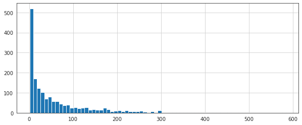
# hist numero di ratings
plt.figure(figsize=(10,4))
ratings['num of ratings'].hist(bins=70)
1
<matplotlib.axes._subplots.AxesSubplot at 0x7fee70493d90>
1
2
3
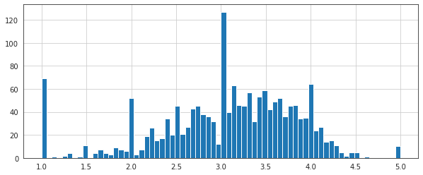
# hist punteggio di rating
plt.figure(figsize=(10,4))
ratings['rating'].hist(bins=70)
1
<matplotlib.axes._subplots.AxesSubplot at 0x7fee73346650>
1
2
3
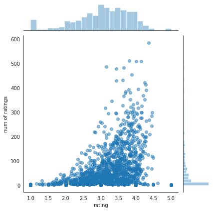
# jointplot punteggio e numero
sns.jointplot(x='rating',y='num of ratings',data=ratings,alpha=0.5)
# i film più belli sono anche quelli più visti e vengono anche più votati
1
<seaborn.axisgrid.JointGrid at 0x7fee83526390>
Recommending Similar Movies by Correlations
1
2
3
# df in formato wide per ogni id
moviemat = df.pivot_table(index='user_id',columns='title',values='rating')
moviemat.head()
| title | 'Til There Was You (1997) | 1-900 (1994) | 101 Dalmatians (1996) | 12 Angry Men (1957) | 187 (1997) | 2 Days in the Valley (1996) | 20,000 Leagues Under the Sea (1954) | 2001: A Space Odyssey (1968) | 3 Ninjas: High Noon At Mega Mountain (1998) | 39 Steps, The (1935) | ... | Yankee Zulu (1994) | Year of the Horse (1997) | You So Crazy (1994) | Young Frankenstein (1974) | Young Guns (1988) | Young Guns II (1990) | Young Poisoner's Handbook, The (1995) | Zeus and Roxanne (1997) | unknown | Á köldum klaka (Cold Fever) (1994) |
|---|---|---|---|---|---|---|---|---|---|---|---|---|---|---|---|---|---|---|---|---|---|
| user_id | |||||||||||||||||||||
| 0 | NaN | NaN | NaN | NaN | NaN | NaN | NaN | NaN | NaN | NaN | ... | NaN | NaN | NaN | NaN | NaN | NaN | NaN | NaN | NaN | NaN |
| 1 | NaN | NaN | 2.0 | 5.0 | NaN | NaN | 3.0 | 4.0 | NaN | NaN | ... | NaN | NaN | NaN | 5.0 | 3.0 | NaN | NaN | NaN | 4.0 | NaN |
| 2 | NaN | NaN | NaN | NaN | NaN | NaN | NaN | NaN | 1.0 | NaN | ... | NaN | NaN | NaN | NaN | NaN | NaN | NaN | NaN | NaN | NaN |
| 3 | NaN | NaN | NaN | NaN | 2.0 | NaN | NaN | NaN | NaN | NaN | ... | NaN | NaN | NaN | NaN | NaN | NaN | NaN | NaN | NaN | NaN |
| 4 | NaN | NaN | NaN | NaN | NaN | NaN | NaN | NaN | NaN | NaN | ... | NaN | NaN | NaN | NaN | NaN | NaN | NaN | NaN | NaN | NaN |
5 rows × 1664 columns
1
2
# most rating movies
ratings.sort_values('num of ratings',ascending=False).head(10)
| rating | num of ratings | |
|---|---|---|
| title | ||
| Star Wars (1977) | 4.359589 | 584 |
| Contact (1997) | 3.803536 | 509 |
| Fargo (1996) | 4.155512 | 508 |
| Return of the Jedi (1983) | 4.007890 | 507 |
| Liar Liar (1997) | 3.156701 | 485 |
| English Patient, The (1996) | 3.656965 | 481 |
| Scream (1996) | 3.441423 | 478 |
| Toy Story (1995) | 3.878319 | 452 |
| Air Force One (1997) | 3.631090 | 431 |
| Independence Day (ID4) (1996) | 3.438228 | 429 |
1
2
3
4
# scelti due film
starwars_user_ratings = moviemat['Star Wars (1977)']
liarliar_user_ratings = moviemat['Liar Liar (1997)']
starwars_user_ratings.head()
1
2
3
4
5
6
7
user_id
0    5.0
1    5.0
2    5.0
3    NaN
4    5.0
Name: Star Wars (1977), dtype: float64
1
2
3
# correlazione il film specifico e gli altri su base clienti
similar_to_starwars = moviemat.corrwith(starwars_user_ratings)
similar_to_liarliar = moviemat.corrwith(liarliar_user_ratings)
1
2
3
4
/home/user/miniconda3/envs/py3/lib/python3.7/site-packages/numpy/lib/function_base.py:2526: RuntimeWarning: Degrees of freedom <= 0 for slice
  c = cov(x, y, rowvar)
/home/user/miniconda3/envs/py3/lib/python3.7/site-packages/numpy/lib/function_base.py:2455: RuntimeWarning: divide by zero encountered in true_divide
  c *= np.true_divide(1, fact)
1
2
# starwars è correlato con til there was you tra gli user id
similar_to_starwars.head()
1
2
3
4
5
6
7
title
'Til There Was You (1997)    0.872872
1-900 (1994)                -0.645497
101 Dalmatians (1996)        0.211132
12 Angry Men (1957)          0.184289
187 (1997)                   0.027398
dtype: float64
1
2
3
4
# formato data frame
corr_starwars = pd.DataFrame(similar_to_starwars,columns=['Correlation'])
corr_starwars.dropna(inplace=True)
corr_starwars.head()
| Correlation | |
|---|---|
| title | |
| 'Til There Was You (1997) | 0.872872 |
| 1-900 (1994) | -0.645497 |
| 101 Dalmatians (1996) | 0.211132 |
| 12 Angry Men (1957) | 0.184289 |
| 187 (1997) | 0.027398 |
1
2
# correlzione a mano tra i due film
pd.concat([starwars_user_ratings,liarliar_user_ratings],axis=1).corr().iloc[[1,],[0]]
| Star Wars (1977) | |
|---|---|
| Liar Liar (1997) | 0.150292 |
1
2
# correlazione estratta dal corrwith
corr_starwars[corr_starwars.index=='Liar Liar (1997)']
| Correlation | |
|---|---|
| title | |
| Liar Liar (1997) | 0.150292 |
1
2
# più correlati con starwars
corr_starwars.sort_values('Correlation',ascending=False).head(10)
| Correlation | |
|---|---|
| title | |
| Hollow Reed (1996) | 1.0 |
| Stripes (1981) | 1.0 |
| Star Wars (1977) | 1.0 |
| Man of the Year (1995) | 1.0 |
| Beans of Egypt, Maine, The (1994) | 1.0 |
| Safe Passage (1994) | 1.0 |
| Old Lady Who Walked in the Sea, The (Vieille qui marchait dans la mer, La) (1991) | 1.0 |
| Outlaw, The (1943) | 1.0 |
| Line King: Al Hirschfeld, The (1996) | 1.0 |
| Hurricane Streets (1998) | 1.0 |
1
2
3
# più correlati con starwars con almeno 100 review
corr_starwars = corr_starwars.join(ratings['num of ratings'])
corr_starwars[corr_starwars['num of ratings']>100].sort_values('Correlation',ascending=False).head()
| Correlation | num of ratings | |
|---|---|---|
| title | ||
| Star Wars (1977) | 1.000000 | 584 |
| Empire Strikes Back, The (1980) | 0.748353 | 368 |
| Return of the Jedi (1983) | 0.672556 | 507 |
| Raiders of the Lost Ark (1981) | 0.536117 | 420 |
| Austin Powers: International Man of Mystery (1997) | 0.377433 | 130 |
1
2
3
4
5
# per liar liar
corr_liarliar = pd.DataFrame(similar_to_liarliar,columns=['Correlation'])
corr_liarliar.dropna(inplace=True)
corr_liarliar = corr_liarliar.join(ratings['num of ratings'])
corr_liarliar[corr_liarliar['num of ratings']>100].sort_values('Correlation',ascending=False).head()
| Correlation | num of ratings | |
|---|---|---|
| title | ||
| Liar Liar (1997) | 1.000000 | 485 |
| Batman Forever (1995) | 0.516968 | 114 |
| Mask, The (1994) | 0.484650 | 129 |
| Down Periscope (1996) | 0.472681 | 101 |
| Con Air (1997) | 0.469828 | 137 |
Collaborative Filtering
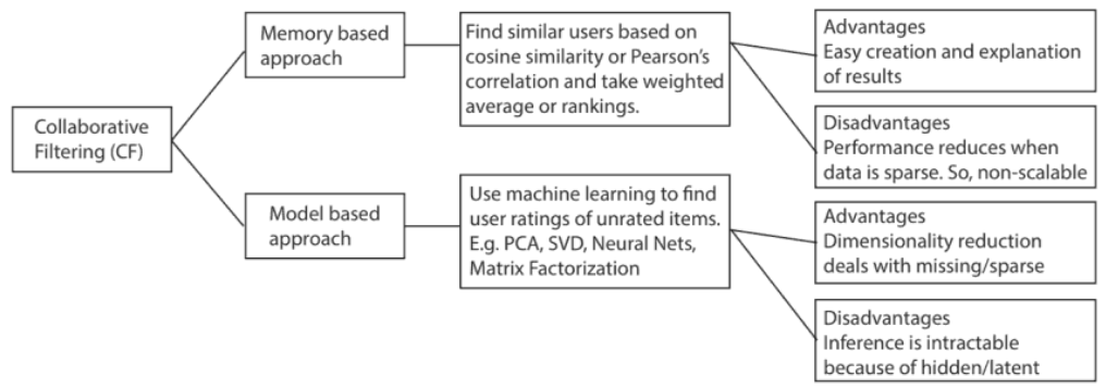
Memory-Based Collaborative Filtering
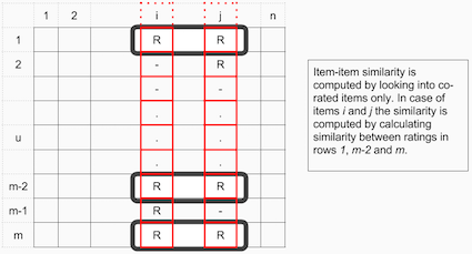
Item-Item Collaborative Filtering: “Users who liked this item also liked …”
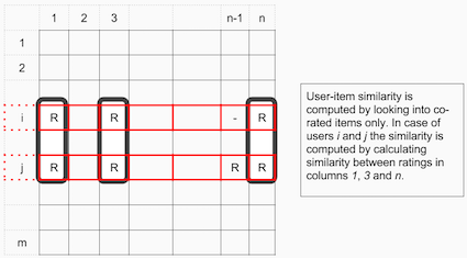
User-Item Collaborative Filtering: “Users who are similar to you also liked …”
1
2
3
4
# train test
train_data, test_data = train_test_split(df, test_size=0.25)
print('Train:', train_data.shape)
print('Test:', test_data.shape)
1
2
Train: (75002, 8)
Test: (25001, 8)
1
2
3
4
5
6
# unique users and movies
n_users = df.user_id.nunique()
n_items = df.item_id.nunique()

print('Num. of Users: '+ str(n_users))
print('Num. of Movies: '+str(n_items))
1
2
Num. of Users: 944
Num. of Movies: 1682
User-Item Matrix
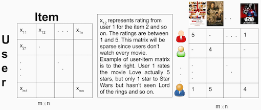
La similarità Item-Item si misura tra utenti che hanno valutato lo stesso film
La similarità User-Item si misura tra i film valutati dagli stessi utenti
Come distance metrics usiamo la cosine similarity
Tra utente k e a, per gli item m e b
\(s_u^{cos}(u_k,u_a)=\frac{u_k \cdot u_a }{ \left \| u_k \right \| \left \| u_a \right \| } =\frac{\sum x_{k,m}x_{a,m}}{\sqrt{\sum x_{k,m}^2\sum x_{a,m}^2}}\)
Tra item m e b, per gli itenti a e k
\(s_u^{cos}(i_m,i_b)=\frac{i_m \cdot i_b }{ \left \| i_m \right \| \left \| i_b \right \| } =\frac{\sum x_{a,m}x_{a,b}}{\sqrt{\sum x_{a,m}^2\sum x_{a,b}^2}}\)
1
2
3
4
5
6
7
8
# creating two user-item matrix (training and test)
train_data_matrix = np.zeros((n_users, n_items))
for line in train_data.itertuples():
    train_data_matrix[line[1]-1, line[2]-1] = line[3]

test_data_matrix = np.zeros((n_users, n_items))
for line in test_data.itertuples():
    test_data_matrix[line[1]-1, line[2]-1] = line[3]
1
2
3
# cosine similarity
user_similarity = pairwise_distances(train_data_matrix, metric='cosine')
item_similarity = pairwise_distances(train_data_matrix.T, metric='cosine')
1
2
3
4
5
6
7
8
9
10
# predictions formula
def predict(ratings, similarity, type='user'):
    if type == 'user':
        mean_user_rating = ratings.mean(axis=1)
        #use np.newaxis so that mean_user_rating has same format as ratings
        ratings_diff = (ratings - mean_user_rating[:, np.newaxis])
        pred = mean_user_rating[:, np.newaxis] + similarity.dot(ratings_diff) / np.array([np.abs(similarity).sum(axis=1)]).T
    elif type == 'item':
        pred = ratings.dot(similarity) / np.array([np.abs(similarity).sum(axis=1)])
    return pred
1
2
3
# prediction
item_prediction = predict(train_data_matrix, item_similarity, type='item')
user_prediction = predict(train_data_matrix, user_similarity, type='user')
Evaluation
Root Mean Squared Error
\(RMSE =\sqrt{\frac{1}{N} \sum (x_i -\hat{x_i})^2}\)
1
2
3
4
5
# RMSE function
def rmse(prediction, ground_truth):
    prediction = prediction[ground_truth.nonzero()].flatten()
    ground_truth = ground_truth[ground_truth.nonzero()].flatten()
    return sqrt(mean_squared_error(prediction, ground_truth))
1
2
3
# metrics
print('User-based CF RMSE: ' + str(rmse(user_prediction, test_data_matrix)))
print('Item-based CF RMSE: ' + str(rmse(item_prediction, test_data_matrix)))
1
2
User-based CF RMSE: 3.144025719792008
Item-based CF RMSE: 3.46950816872225
Model-Based Collaborative Filtering
Based on matrix factorization (MF). The goal of MF is to learn the latent preferences of users and the latent attributes of items from known ratings (learn features that describe the characteristics of ratings) to then predict the unknown ratings through the dot product of the latent features of users and items.
You can represent a very sparse matrix by the multiplication of two low-rank matrics, where the rows contain the latent vector.
It’s better to use Hybrid Recommender Systems to mix CF and CB models to improve cold-start problem since you have no ratings.
1
2
3
# Sparsity level of MovieLens dataset
sparsity=round(1.0-len(df)/float(n_users*n_items),3)
print('The sparsity level of MovieLens100K is ' +  str(sparsity*100) + '%')
1
The sparsity level of MovieLens100K is 93.7%
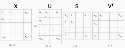
Singular Value Decomposition
\(X=USV^T\) Given m x n matrix X:
- U is an (m x r) orthogonal matrix
- S is an (r x r) diagonal matrix with non-negative real numbers on the diagonal
- V^T is an (r x n) orthogonal matrix
1
2
3
4
5
# get SVD components from train matrix. Choose k.
u, s, vt = svds(train_data_matrix, k = 20)
s_diag_matrix=np.diag(s)
X_pred = np.dot(np.dot(u, s_diag_matrix), vt)
print('User-based CF MSE: ' + str(rmse(X_pred, test_data_matrix)))
1
User-based CF MSE: 2.729577819518798
More resources
Movies Recommendation:
MovieLens - Movie Recommendation Data Sets
Yahoo! - Movie, Music, and Images Ratings Data Sets
Jester - Movie Ratings Data Sets (Collaborative Filtering Dataset)
Cornell University - Movie-review data for use in sentiment-analysis experiments
Music Recommendation:
Last.fm - Music Recommendation Data Sets
Yahoo! - Movie, Music, and Images Ratings Data Sets
Audioscrobbler - Music Recommendation Data Sets
Amazon - Audio CD recommendations
Books Recommendation:
Institut für Informatik, Universität Freiburg - Book Ratings Data Sets
Food Recommendation:
Chicago Entree - Food Ratings Data Sets
Healthcare Recommendation:
Nursing Home - Provider Ratings Data Set
Hospital Ratings - Survey of Patients Hospital Experiences
Dating Recommendation:
www.libimseti.cz - Dating website recommendation (collaborative filtering)
Scholarly Paper Recommendation:
National University of Singapore - Scholarly Paper Recommendation