Python: Tree and Random Forest
Utilizzo l’environment conda py3
1
~$ conda activate py3
Versione modulo installato
1
2
3
4
5
6
7
8
9
10
11
12
~$ pip show pydot
Name: scikit-learn
Name: pydot
Version: 1.4.1
Summary: Python interface to Graphviz's Dot
Home-page: https://github.com/pydot/pydot
Author: Ero Carrera
Author-email: ero@dkbza.org
License: MIT
Location: /home/user/miniconda3/envs/py3/lib/python3.7/site-packages
Requires: pyparsing
Required-by:
Tree Methods
Decision Tree

Se si usa l’algoritmo ID3, lo split deve massimizzare l’Information Gain
Entropy
\(H\left (S\right )=-\sum_{i}p_{i}\left (S\right)\log_{2}p_{i}\left (S\right )\)
Information Gain
\(IG\left (S,A\right )=H\left (S\right )-\sum_{\nu \in Values\left (A\right )}\frac{\left | S_{\nu}\right |}{S}H\left (S_{\nu}\right )=H\left (S\right )-H\left (S,A\right )\)
Random Forest
Bootstrapping rows and sampling columns every tree is generated.
1
2
3
4
5
6
7
8
9
10
11
12
13
14
15
16
17
# lib
import pandas as pd
import numpy as np
import matplotlib.pyplot as plt
import seaborn as sns
%matplotlib inline

from sklearn.model_selection import train_test_split
from sklearn.tree import DecisionTreeClassifier
from sklearn.metrics import classification_report,confusion_matrix

from IPython.display import Image
from six import StringIO
from sklearn.tree import export_graphviz
import pydot

from sklearn.ensemble import RandomForestClassifier
1
2
3
# data
df = pd.read_csv(r'kyphosis.csv')
df.head()
| Kyphosis | Age | Number | Start | |
|---|---|---|---|---|
| 0 | absent | 71 | 3 | 5 |
| 1 | absent | 158 | 3 | 14 |
| 2 | present | 128 | 4 | 5 |
| 3 | absent | 2 | 5 | 1 |
| 4 | absent | 1 | 4 | 15 |
1
2
3
4
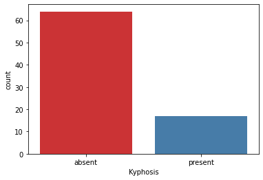
# distribuzione target
print(df['Kyphosis'].value_counts())
sns.countplot(x='Kyphosis',data=df,palette='Set1') # palette='RdBu_r'
# è abbastanza sbilanciato
1
2
3
4
5
absent     64
present    17
Name: Kyphosis, dtype: int64

<matplotlib.axes._subplots.AxesSubplot at 0x7f03c04281d0>
1
df.info()
1
2
3
4
5
6
7
8
9
10
11
<class 'pandas.core.frame.DataFrame'>
RangeIndex: 81 entries, 0 to 80
Data columns (total 4 columns):
 #   Column    Non-Null Count  Dtype
---  ------    --------------  -----
 0   Kyphosis  81 non-null     object
 1   Age       81 non-null     int64
 2   Number    81 non-null     int64
 3   Start     81 non-null     int64
dtypes: int64(3), object(1)
memory usage: 2.7+ KB
1
2
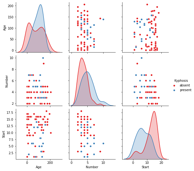
# pairplot
sns.pairplot(df,hue='Kyphosis',palette='Set1')
1
<seaborn.axisgrid.PairGrid at 0x7f03cc1a2290>
1
2
3
4
# train test split
X = df.drop('Kyphosis',axis=1)
y = df['Kyphosis']
X_train, X_test, y_train, y_test = train_test_split(X, y, test_size=0.30)
Decision Tree
1
2
3
# tree
dtree = DecisionTreeClassifier()
dtree.fit(X_train,y_train)
1
DecisionTreeClassifier()
1
2
# predictions
predictions = dtree.predict(X_test)
1
2
3
4
5
# confusion matrix and classification metrix
print('\nConfusion Matrix:')
print(confusion_matrix(y_test,predictions))
print('\nClassification metrics:')
print(classification_report(y_test,predictions))
1
2
3
4
5
6
7
8
9
10
11
12
13
Confusion Matrix:
[[17  2]
 [ 2  4]]

Classification metrics:
              precision    recall  f1-score   support

      absent       0.89      0.89      0.89        19
     present       0.67      0.67      0.67         6

    accuracy                           0.84        25
   macro avg       0.78      0.78      0.78        25
weighted avg       0.84      0.84      0.84        25
Tree Visualization
1
2
3
# cols
features = list(df.columns[1:])
features
1
['Age', 'Number', 'Start']
1
2
3
4
5
6
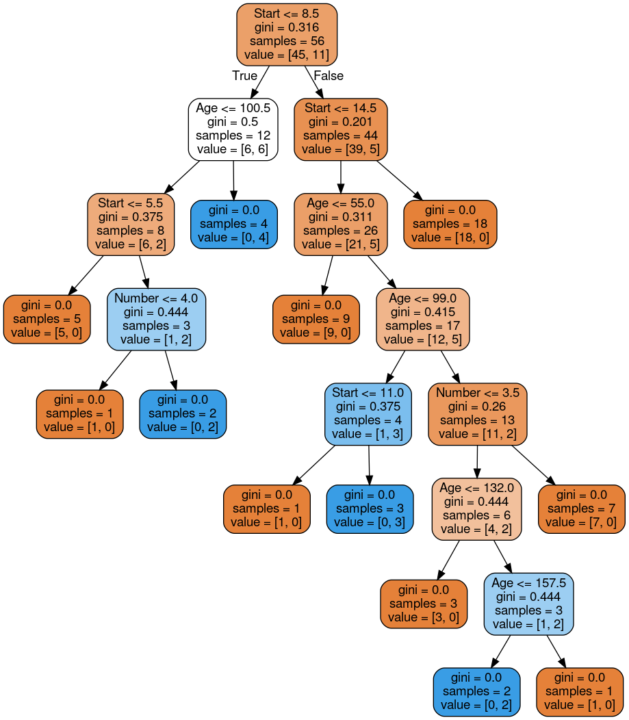
# plot tree
dot_data = StringIO()
export_graphviz(dtree, out_file=dot_data,feature_names=features,filled=True,rounded=True)
graph = pydot.graph_from_dot_data(dot_data.getvalue())
Image(graph[0].create_png())
Random Forest
1
2
3
# RF
rfc = RandomForestClassifier(n_estimators=300)
rfc.fit(X_train, y_train)
1
RandomForestClassifier(n_estimators=300)
1
2
# predictions
rfc_pred = rfc.predict(X_test)
1
2
3
4
5
# confusion matrix and classification metrix
print('\nConfusion Matrix:')
print(confusion_matrix(y_test,rfc_pred))
print('\nClassification metrics:')
print(classification_report(y_test,rfc_pred))
1
2
3
4
5
6
7
8
9
10
11
12
13
Confusion Matrix:
[[18  1]
 [ 3  3]]

Classification metrics:
              precision    recall  f1-score   support

      absent       0.86      0.95      0.90        19
     present       0.75      0.50      0.60         6

    accuracy                           0.84        25
   macro avg       0.80      0.72      0.75        25
weighted avg       0.83      0.84      0.83        25
Altro
Better confusion matrix
1
2
3
4
5
# matrice per absent è yes
pd.DataFrame(confusion_matrix(y_test,rfc_pred, labels=['absent', 'present']),
             index=['TRUE | Yes', 'TRUE | No'],
             columns=['PRED | Yes', 'PRED | No'])
# esempio: precision per absent è 18/(18+3)=0.86
| PRED | Yes | PRED | No | |
|---|---|---|
| TRUE | Yes | 18 | 1 |
| TRUE | No | 3 | 3 |
1
2
3
4
5
# matrice per present è yes
pd.DataFrame(confusion_matrix(y_test,rfc_pred, labels=['present','absent']),
             index=['TRUE | Yes', 'TRUE | No'],
             columns=['PRED | Yes', 'PRED | No'])
# esempio: recall per present è 3/(3+3)=0.5
| PRED | Yes | PRED | No | |
|---|---|---|
| TRUE | Yes | 3 | 3 |
| TRUE | No | 1 | 18 |
1
2
3
4
5
6
7
8
9
10
# costruisco una funzione
def confusion_matrix_bella(y_true, y_pred, labels='default'):
    if labels is 'default':
        labels = np.unique([y_true,y_pred])
    cmtx = pd.DataFrame(
        confusion_matrix(y_true, y_pred, labels=labels),
        index=['TRUE | {:}'.format(x) for x in labels],
        columns=['PRED | {:}'.format(x) for x in labels]
    )
    return(cmtx)
1
confusion_matrix_bella(y_test,rfc_pred,labels=['absent','present'])
| PRED | present | PRED | absent | |
|---|---|---|
| TRUE | present | 3 | 3 |
| TRUE | absent | 1 | 18 |
Better distplot
1
2
3
4
5
6
7
8
9
10
11
12
# better displot function
def distplot_fig(data, x, hue=None, row=None, col=None, height=3, aspect=1, legend=True, hist=False, **kwargs):
    """A figure-level distribution plot with support for hue, col, row arguments."""
    bins = kwargs.pop('bins', None)
    if (bins is None) and hist:
        # Make sure that the groups have equal-sized bins
        bins = np.histogram_bin_edges(data[x].dropna())
    g = sns.FacetGrid(data, hue=hue, row=row, col=col, height=height, aspect=aspect)
    g.map(sns.distplot, x, bins=bins, hist=hist, **kwargs)
    if legend and (hue is not None) and (hue not in [x, row, col]):
        g.add_legend(title=hue)
    return g
1
2
# better distplot
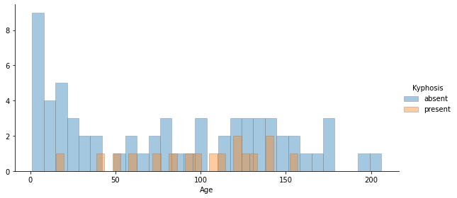
distplot_fig(data=df,x='Age',hue='Kyphosis',kde=False,hist=True,hist_kws=dict(edgecolor='grey'),bins=30, height=4, aspect=2)
1
<seaborn.axisgrid.FacetGrid at 0x7f03c05ee910>
1
2
3
4
5
# multiple displot (seaborn)
plt.figure(figsize=(10,6))
sns.distplot(df[df['Kyphosis']=='absent']['Age'],kde=False,color='b',bins=20,hist_kws=dict(edgecolor='grey'),label='Kyphosis = absent')
sns.distplot(df[df['Kyphosis']=='present']['Age'],kde=False,color='y',bins=20,hist_kws=dict(edgecolor='grey'),label='Kyphosis = present')
plt.legend()
1
<matplotlib.legend.Legend at 0x7f03c9a55550>

1
2
3
4
5
6
7
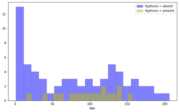
# multiple distplot (matplotlib)
plt.figure(figsize=(10,6))
df[df['Kyphosis']=='absent']['Age'].hist(alpha=0.5,color='b',bins=20,label='Kyphosis = absent',edgecolor="grey")
df[df['Kyphosis']=='present']['Age'].hist(alpha=0.5,color='y',bins=20,label='Kyphosis = present',edgecolor="grey")
plt.legend()
plt.xlabel('Age')
plt.grid(None)