
Python: Logistic Regression
Utilizzo l’environment conda py3
1
2
~$ conda activate py3
~$ conda deactivate
Logistic Regression
Sigmoid o Logistic
\[\forall x \in \mathbb{R} \\ f\left (x\right ) \in \left [0,1\right ] \\ f\left (x\right )=\frac{1}{1+e^{-x}}=\frac{e^{x}}{e^{x}+1}\]Linear regression to Logistic
\[y=b_{0}+b_{1}\cdot x \\ p=\frac{1}{1+e^{-\left (b_{0}+b_{1}\cdot x\right )}}\]Titanic dataset
1
2
3
4
5
6
7
8
9
10
11
# lib
import pandas as pd
import numpy as np
import matplotlib.pyplot as plt
import seaborn as sns
%matplotlib inline

from sklearn.model_selection import train_test_split
from sklearn.linear_model import LogisticRegression
from sklearn.metrics import classification_report
from sklearn.metrics import confusion_matrix
1
2
3
# train df
train = pd.read_csv('titanic_train.csv')
train.head()
| PassengerId | Survived | Pclass | Name | Sex | Age | SibSp | Parch | Ticket | Fare | Cabin | Embarked | |
|---|---|---|---|---|---|---|---|---|---|---|---|---|
| 0 | 1 | 0 | 3 | Braund, Mr. Owen Harris | male | 22.0 | 1 | 0 | A/5 21171 | 7.2500 | NaN | S |
| 1 | 2 | 1 | 1 | Cumings, Mrs. John Bradley (Florence Briggs Th... | female | 38.0 | 1 | 0 | PC 17599 | 71.2833 | C85 | C |
| 2 | 3 | 1 | 3 | Heikkinen, Miss. Laina | female | 26.0 | 0 | 0 | STON/O2. 3101282 | 7.9250 | NaN | S |
| 3 | 4 | 1 | 1 | Futrelle, Mrs. Jacques Heath (Lily May Peel) | female | 35.0 | 1 | 0 | 113803 | 53.1000 | C123 | S |
| 4 | 5 | 0 | 3 | Allen, Mr. William Henry | male | 35.0 | 0 | 0 | 373450 | 8.0500 | NaN | S |
1
train.info()
1
2
3
4
5
6
7
8
9
10
11
12
13
14
15
16
17
18
19
<class 'pandas.core.frame.DataFrame'>
RangeIndex: 891 entries, 0 to 890
Data columns (total 12 columns):
 #   Column       Non-Null Count  Dtype
---  ------       --------------  -----
 0   PassengerId  891 non-null    int64
 1   Survived     891 non-null    int64
 2   Pclass       891 non-null    int64
 3   Name         891 non-null    object
 4   Sex          891 non-null    object
 5   Age          714 non-null    float64
 6   SibSp        891 non-null    int64
 7   Parch        891 non-null    int64
 8   Ticket       891 non-null    object
 9   Fare         891 non-null    float64
 10  Cabin        204 non-null    object
 11  Embarked     889 non-null    object
dtypes: float64(2), int64(5), object(5)
memory usage: 83.7+ KB
1
train.describe()
| Survived | Pclass | Age | SibSp | Parch | Fare | Sex_male | Embarked_Q | Embarked_S | |
|---|---|---|---|---|---|---|---|---|---|
| count | 889.000000 | 889.000000 | 889.000000 | 889.000000 | 889.000000 | 889.000000 | 889.000000 | 889.000000 | 889.000000 |
| mean | 0.382452 | 2.311586 | 29.019314 | 0.524184 | 0.382452 | 32.096681 | 0.649044 | 0.086614 | 0.724409 |
| std | 0.486260 | 0.834700 | 13.209814 | 1.103705 | 0.806761 | 49.697504 | 0.477538 | 0.281427 | 0.447063 |
| min | 0.000000 | 1.000000 | 0.420000 | 0.000000 | 0.000000 | 0.000000 | 0.000000 | 0.000000 | 0.000000 |
| 25% | 0.000000 | 2.000000 | 22.000000 | 0.000000 | 0.000000 | 7.895800 | 0.000000 | 0.000000 | 0.000000 |
| 50% | 0.000000 | 3.000000 | 26.000000 | 0.000000 | 0.000000 | 14.454200 | 1.000000 | 0.000000 | 1.000000 |
| 75% | 1.000000 | 3.000000 | 36.500000 | 1.000000 | 0.000000 | 31.000000 | 1.000000 | 0.000000 | 1.000000 |
| max | 1.000000 | 3.000000 | 80.000000 | 8.000000 | 6.000000 | 512.329200 | 1.000000 | 1.000000 | 1.000000 |
EDA
1
2
3
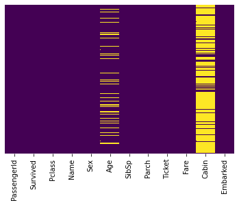
# view missing data
sns.heatmap(train.isnull(),yticklabels=False,cbar=False,cmap='viridis')
# maybe we will fill age and dropping cabin
1
<matplotlib.axes._subplots.AxesSubplot at 0x7fb227a84590>
1
2
3
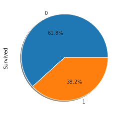
# target distribution
sns.set_style('whitegrid')
train['Survived'].value_counts().plot.pie(autopct='%1.1f%%',shadow=True,figsize=(4,4))
1
<matplotlib.axes._subplots.AxesSubplot at 0x7fb222c5bb50>
1
2
3
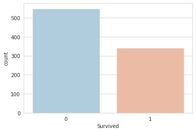
# target distribution
sns.set_style('whitegrid')
sns.countplot(x='Survived',data=train,palette='RdBu_r')
1
<matplotlib.axes._subplots.AxesSubplot at 0x7fb22728c110>
1
2
3
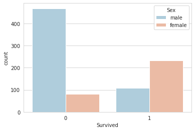
# target barplot stratified with sex
sns.set_style('whitegrid')
sns.countplot(x='Survived',hue='Sex',data=train,palette='RdBu_r')
1
<matplotlib.axes._subplots.AxesSubplot at 0x7fb2271fff50>
1
2
3
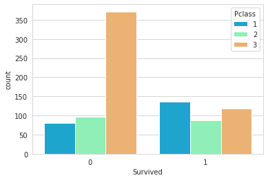
# target barplot stratified with passenger class
sns.set_style('whitegrid')
sns.countplot(x='Survived',hue='Pclass',data=train,palette='rainbow')
1
<matplotlib.axes._subplots.AxesSubplot at 0x7fb227176150>
1
2
3
4
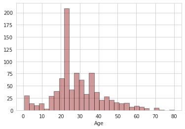
# eta histogram
sns.distplot(train['Age'].dropna(),kde=False,color='darkred',bins=30,hist_kws=dict(edgecolor="black", linewidth=1))
# train['Age'].hist(bins=30,color='darkred',alpha=0.7,edgecolor='black', linewidth=1)
# plt.xlabel('Age')
1
<matplotlib.axes._subplots.AxesSubplot at 0x7fb2235ae310>
1
2
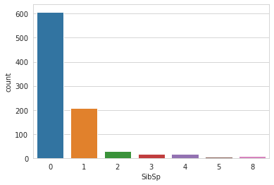
# barplot of number of siblings or spouse
sns.countplot(x='SibSp',data=train)
1
<matplotlib.axes._subplots.AxesSubplot at 0x7fb227045890>
1
2
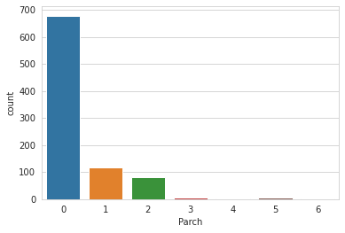
# barplot of number of parents or children
sns.countplot(x='Parch',data=train)
1
<matplotlib.axes._subplots.AxesSubplot at 0x7fb226fb23d0>
1
2
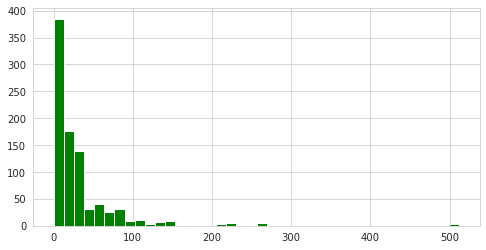
# histogram of price of the ticket
train['Fare'].hist(color='green',bins=40,figsize=(8,4))
1
<matplotlib.axes._subplots.AxesSubplot at 0x7fb226ea7990>
Data Cleaning
1
2
3
4
5
6
7
8
9
10
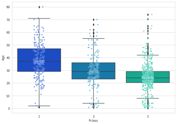
# boxplot passenger class and age
# plt.figure(figsize=(12, 7))
# sns.boxplot(x='Pclass',y='Age',data=train,palette='winter')
# object oriented
fig = plt.figure() # .figure() create a new figure whereas .gcf() stands for get current figure
fig.set_size_inches(10,7)
fig = sns.boxplot(x='Pclass',y='Age',data=train,palette='winter')
fig = sns.stripplot(x='Pclass',y='Age',data=train,jitter=True,edgecolor='white',alpha=0.5,linewidth=1,palette='winter')
plt.show()
# la prima classe ha mediamente un'età più avanzata
1
2
3
4
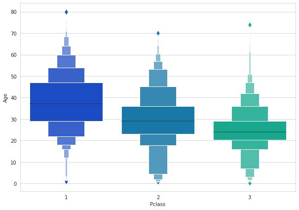
# Boxen Plot
fig=plt.gcf()
fig.set_size_inches(10,7)
fig=sns.boxenplot(x='Pclass',y='Age',data=train,palette='winter')
1
2
3
4
5
6
7
8
9
10
11
12
13
14
15
16
17
18
19
20
21
22
23
# imputare i missing dell'età
# funzione
def impute_age(cols):
    Age = cols[0]
    Pclass = cols[1]

    if pd.isnull(Age):

        if Pclass == 1:
            return 37

        elif Pclass == 2:
            return 29

        else:
            return 24

    else:
        return Age
# assegnazione
print("Pre imputazione:", train['Age'].isnull().sum())
train['Age'] = train[['Age','Pclass']].apply(impute_age,axis=1)
print("Post imputazione:", train['Age'].isnull().sum())
1
2
Pre imputazione: 177
Post imputazione: 0
1
2
# esclusione cabin
train.drop('Cabin',axis=1,inplace=True)
1
2
3
4
# esclusione record missing
print("Pre esclusione record missing:", len(train))
train.dropna(inplace=True)
print("Post esclusione record missing:", len(train))
1
2
Pre esclusione record missing: 891
Post esclusione record missing: 889
1
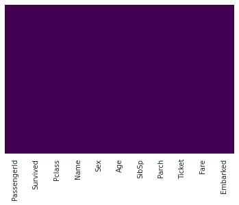
2
# view missing data
sns.heatmap(train.isnull(),yticklabels=False,cbar=False,cmap='viridis')
1
<matplotlib.axes._subplots.AxesSubplot at 0x7fb223f2a050>
OneHotEncoding/Dummyfication/Dummy Categorical features
1
train.info()
1
2
3
4
5
6
7
8
9
10
11
12
13
14
15
16
17
18
<class 'pandas.core.frame.DataFrame'>
Int64Index: 889 entries, 0 to 890
Data columns (total 11 columns):
 #   Column       Non-Null Count  Dtype
---  ------       --------------  -----
 0   PassengerId  889 non-null    int64
 1   Survived     889 non-null    int64
 2   Pclass       889 non-null    int64
 3   Name         889 non-null    object
 4   Sex          889 non-null    object
 5   Age          889 non-null    float64
 6   SibSp        889 non-null    int64
 7   Parch        889 non-null    int64
 8   Ticket       889 non-null    object
 9   Fare         889 non-null    float64
 10  Embarked     889 non-null    object
dtypes: float64(2), int64(5), object(4)
memory usage: 83.3+ KB
1
2
3
4
5
6
7
8
9
10
11
12
13
14
15
# dummy
sex = pd.get_dummies(train['Sex'],drop_first=True,prefix='Sex')
embark = pd.get_dummies(train['Embarked'],drop_first=True,prefix='Embarked')

# invece di costruirle singolarmente, si possono dummificare tutte in un record
# train = pd.get_dummies(train,columns=['Sex','Embarked'],drop_first=True)

# escludo variabili inutili
train.drop(['Sex','Embarked','Name','Ticket','PassengerId'],axis=1,inplace=True)

# aggiungo le dummy create
train = pd.concat([train,sex,embark],axis=1)

# head
train.head()
| Survived | Pclass | Age | SibSp | Parch | Fare | Sex_male | Embarked_Q | Embarked_S | |
|---|---|---|---|---|---|---|---|---|---|
| 0 | 0 | 3 | 22.0 | 1 | 0 | 7.2500 | 1 | 0 | 1 |
| 1 | 1 | 1 | 38.0 | 1 | 0 | 71.2833 | 0 | 0 | 0 |
| 2 | 1 | 3 | 26.0 | 0 | 0 | 7.9250 | 0 | 0 | 1 |
| 3 | 1 | 1 | 35.0 | 1 | 0 | 53.1000 | 0 | 0 | 1 |
| 4 | 0 | 3 | 35.0 | 0 | 0 | 8.0500 | 1 | 0 | 1 |
Logistic Regression
1
2
# train test
X_train, X_test, y_train, y_test = train_test_split(train.drop('Survived',axis=1),train['Survived'], test_size=0.30,random_state=101)
1
2
3
4
# model
logmodel = LogisticRegression(max_iter=10000)
# the solver was "liblinear" now it is "lbfgs" and needs more iterations
logmodel.fit(X_train,y_train)
1
LogisticRegression(max_iter=10000)
1
2
# prediction
predictions = logmodel.predict(X_test)
1
2
# evaluation report
print(classification_report(y_test,predictions))
1
2
3
4
5
6
7
8
              precision    recall  f1-score   support

           0       0.82      0.92      0.87       163
           1       0.85      0.69      0.76       104

    accuracy                           0.83       267
   macro avg       0.84      0.81      0.82       267
weighted avg       0.83      0.83      0.83       267
1
2
# confusion matrix
print(confusion_matrix(y_test,predictions))
1
2
[[150  13]
 [ 32  72]]
Improvements
- Try grabbing the Title (Dr.,Mr.,Mrs,etc..) from the name as a feature
- Maybe the Cabin letter could be a feature
- Is there any info you can get from the ticket?
- Evaluate the model on the test data (after clearing it)