
Python: Linear Regression
Utilizzo l’environment conda py3
1
~$ conda activate py3
Versione modulo installato
1
2
3
4
5
6
7
8
9
10
11
~$ pip show scikit-learn
Name: scikit-learn
Version: 0.23.1
Summary: A set of python modules for machine learning and data mining
Home-page: http://scikit-learn.org
Author: None
Author-email: None
License: new BSD
Location: /home/user/miniconda3/envs/py3/lib/python3.7/site-packages
Requires: scipy, joblib, threadpoolctl, numpy
Required-by:
USA Housing
1
2
3
4
5
import pandas as pd
import numpy as np
import matplotlib.pyplot as plt
import seaborn as sns
%matplotlib inline
1
2
3
# data
USAhousing = pd.read_csv('USA_Housing.csv')
USAhousing.head()
| Avg. Area Income | Avg. Area House Age | Avg. Area Number of Rooms | Avg. Area Number of Bedrooms | Area Population | Price | Address | |
|---|---|---|---|---|---|---|---|
| 0 | 79545.458574 | 5.682861 | 7.009188 | 4.09 | 23086.800503 | 1.059034e+06 | 208 Michael Ferry Apt. 674\nLaurabury, NE 3701... |
| 1 | 79248.642455 | 6.002900 | 6.730821 | 3.09 | 40173.072174 | 1.505891e+06 | 188 Johnson Views Suite 079\nLake Kathleen, CA... |
| 2 | 61287.067179 | 5.865890 | 8.512727 | 5.13 | 36882.159400 | 1.058988e+06 | 9127 Elizabeth Stravenue\nDanieltown, WI 06482... |
| 3 | 63345.240046 | 7.188236 | 5.586729 | 3.26 | 34310.242831 | 1.260617e+06 | USS Barnett\nFPO AP 44820 |
| 4 | 59982.197226 | 5.040555 | 7.839388 | 4.23 | 26354.109472 | 6.309435e+05 | USNS Raymond\nFPO AE 09386 |
EDA
1
USAhousing.info()
1
2
3
4
5
6
7
8
9
10
11
12
13
14
<class 'pandas.core.frame.DataFrame'>
RangeIndex: 5000 entries, 0 to 4999
Data columns (total 7 columns):
 #   Column                        Non-Null Count  Dtype
---  ------                        --------------  -----
 0   Avg. Area Income              5000 non-null   float64
 1   Avg. Area House Age           5000 non-null   float64
 2   Avg. Area Number of Rooms     5000 non-null   float64
 3   Avg. Area Number of Bedrooms  5000 non-null   float64
 4   Area Population               5000 non-null   float64
 5   Price                         5000 non-null   float64
 6   Address                       5000 non-null   object
dtypes: float64(6), object(1)
memory usage: 273.6+ KB
1
2
# statistiche
USAhousing.describe()
| Avg. Area Income | Avg. Area House Age | Avg. Area Number of Rooms | Avg. Area Number of Bedrooms | Area Population | Price | |
|---|---|---|---|---|---|---|
| count | 5000.000000 | 5000.000000 | 5000.000000 | 5000.000000 | 5000.000000 | 5.000000e+03 |
| mean | 68583.108984 | 5.977222 | 6.987792 | 3.981330 | 36163.516039 | 1.232073e+06 |
| std | 10657.991214 | 0.991456 | 1.005833 | 1.234137 | 9925.650114 | 3.531176e+05 |
| min | 17796.631190 | 2.644304 | 3.236194 | 2.000000 | 172.610686 | 1.593866e+04 |
| 25% | 61480.562388 | 5.322283 | 6.299250 | 3.140000 | 29403.928702 | 9.975771e+05 |
| 50% | 68804.286404 | 5.970429 | 7.002902 | 4.050000 | 36199.406689 | 1.232669e+06 |
| 75% | 75783.338666 | 6.650808 | 7.665871 | 4.490000 | 42861.290769 | 1.471210e+06 |
| max | 107701.748378 | 9.519088 | 10.759588 | 6.500000 | 69621.713378 | 2.469066e+06 |
1
2
# nomi colonne
USAhousing.columns
1
2
3
Index(['Avg. Area Income', 'Avg. Area House Age', 'Avg. Area Number of Rooms',
       'Avg. Area Number of Bedrooms', 'Area Population', 'Price', 'Address'],
      dtype='object')
1
2
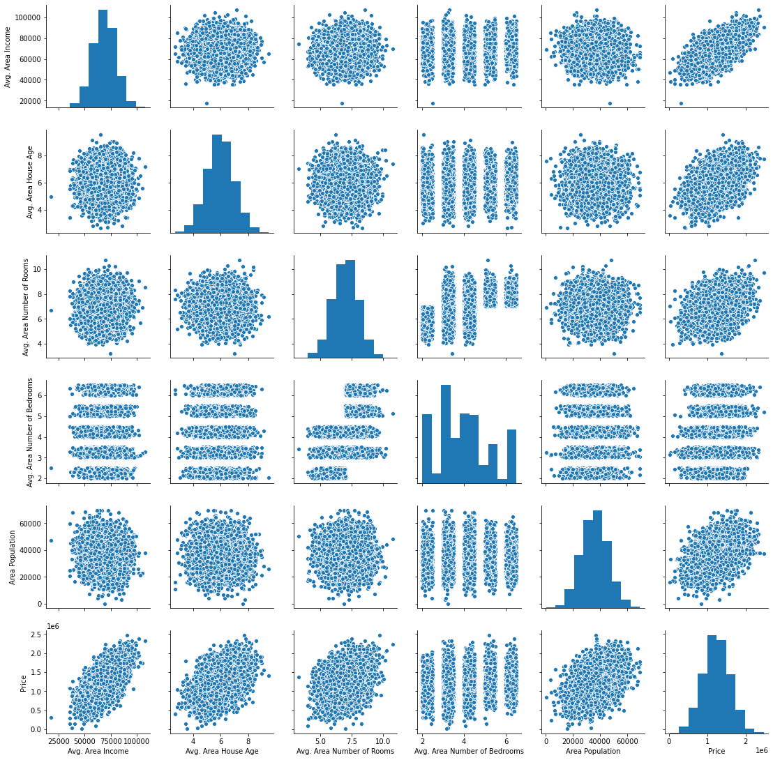
# pairplot
sns.pairplot(USAhousing)
1
<seaborn.axisgrid.PairGrid at 0x7ffba0e6db50>
1
2
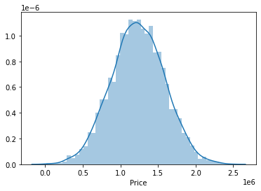
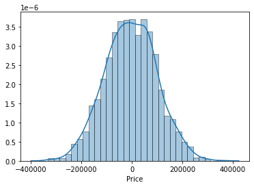
# price distribution
sns.distplot(USAhousing['Price'])
1
<matplotlib.axes._subplots.AxesSubplot at 0x7ffb7646ef10>
1
2
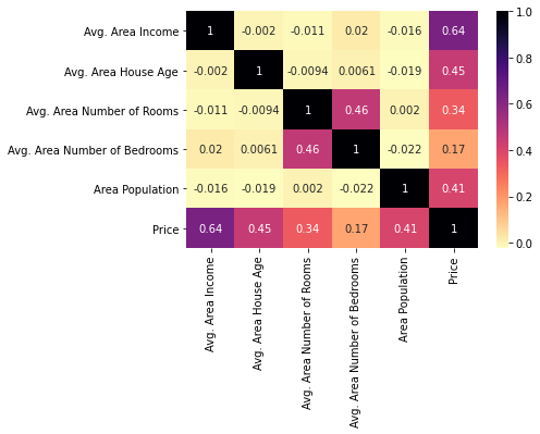
# heatmap
sns.heatmap(USAhousing.corr(), cmap='magma_r', annot=True)
1
<matplotlib.axes._subplots.AxesSubplot at 0x7ffb7645cb50>
Training Model
1
2
3
4
# sklearn
from sklearn.model_selection import train_test_split
from sklearn.linear_model import LinearRegression
from sklearn import metrics
1
2
3
# X e y
X = USAhousing[['Avg. Area Income', 'Avg. Area House Age', 'Avg. Area Number of Rooms','Avg. Area Number of Bedrooms', 'Area Population']]
y = USAhousing['Price']
1
2
# train e test set
X_train, X_test, y_train, y_test = train_test_split(X, y, test_size=0.4, random_state=101)
1
2
3
# train model
lm = LinearRegression()
lm.fit(X_train,y_train)
1
LinearRegression()
1
2
# intercept
print(lm.intercept_)
1
-2640159.7968526687
1
2
3
# coefficients
coeff_df = pd.DataFrame(data=lm.coef_,index=X.columns,columns=['Coefficient'])
coeff_df
| Coefficient | |
|---|---|
| Avg. Area Income | 21.528276 |
| Avg. Area House Age | 164883.282027 |
| Avg. Area Number of Rooms | 122368.678027 |
| Avg. Area Number of Bedrooms | 2233.801864 |
| Area Population | 15.150420 |
Predictions
1
predictions = lm.predict(X_test)
1
2
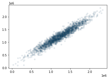
# scatterplot predictions
plt.scatter(y_test,predictions,marker='o',edgecolors='black',alpha=0.1,s=20)
1
<matplotlib.collections.PathCollection at 0x7ffb572f8f50>
1
2
# distplot residuals
sns.distplot(y_test-predictions,bins=30, hist_kws=dict(edgecolor="black", linewidth=1))
1
<matplotlib.axes._subplots.AxesSubplot at 0x7ffb56de2a10>
Metrics
1
2
3
print('MAE:', metrics.mean_absolute_error(y_test, predictions))
print('MSE:', metrics.mean_squared_error(y_test, predictions))
print('RMSE:', np.sqrt(metrics.mean_squared_error(y_test, predictions)))
1
2
3
MAE: 82288.22251914944
MSE: 10460958907.208954
RMSE: 102278.82922290885
1
2
# Explained Variance Score (R^2)
metrics.explained_variance_score(y_test,predictions)
1
0.9178179926151842
Boston dataset
1
2
3
4
5
# df su cui giocare
from sklearn.datasets import load_boston
boston = load_boston()
print(boston.DESCR)
boston_df = boston.data
1
2
3
4
5
6
7
8
9
10
11
12
13
14
15
16
17
18
19
20
21
22
23
24
25
26
27
28
29
30
31
32
33
34
35
36
37
38
39
40
41
42
43
44
45
46
47
48
49
50
.. _boston_dataset:

Boston house prices dataset
---------------------------

**Data Set Characteristics:**

    :Number of Instances: 506

    :Number of Attributes: 13 numeric/categorical predictive. Median Value (attribute 14) is usually the target.

    :Attribute Information (in order):
        - CRIM     per capita crime rate by town
        - ZN       proportion of residential land zoned for lots over 25,000 sq.ft.
        - INDUS    proportion of non-retail business acres per town
        - CHAS     Charles River dummy variable (= 1 if tract bounds river; 0 otherwise)
        - NOX      nitric oxides concentration (parts per 10 million)
        - RM       average number of rooms per dwelling
        - AGE      proportion of owner-occupied units built prior to 1940
        - DIS      weighted distances to five Boston employment centres
        - RAD      index of accessibility to radial highways
        - TAX      full-value property-tax rate per $10,000
        - PTRATIO  pupil-teacher ratio by town
        - B        1000(Bk - 0.63)^2 where Bk is the proportion of blacks by town
        - LSTAT    % lower status of the population
        - MEDV     Median value of owner-occupied homes in $1000's

    :Missing Attribute Values: None

    :Creator: Harrison, D. and Rubinfeld, D.L.

This is a copy of UCI ML housing dataset.
https://archive.ics.uci.edu/ml/machine-learning-databases/housing/


This dataset was taken from the StatLib library which is maintained at Carnegie Mellon University.

The Boston house-price data of Harrison, D. and Rubinfeld, D.L. 'Hedonic
prices and the demand for clean air', J. Environ. Economics & Management,
vol.5, 81-102, 1978.   Used in Belsley, Kuh & Welsch, 'Regression diagnostics
...', Wiley, 1980.   N.B. Various transformations are used in the table on
pages 244-261 of the latter.

The Boston house-price data has been used in many machine learning papers that address regression
problems.

.. topic:: References

   - Belsley, Kuh & Welsch, 'Regression diagnostics: Identifying Influential Data and Sources of Collinearity', Wiley, 1980. 244-261.
   - Quinlan,R. (1993). Combining Instance-Based and Model-Based Learning. In Proceedings on the Tenth International Conference of Machine Learning, 236-243, University of Massachusetts, Amherst. Morgan Kaufmann.