
Python: Neural Networks
Scritto ed eseguito sul portatile con Windows 10 – Effetto South Working
Utilizzo l’environment conda py3_tf
1
~$ conda activate py3_tf
Versione modulo installato
1
2
3
4
5
6
7
8
9
10
11
~$ pip show tensorflow
Name: tensorflow
Version: 2.2.0
Summary: TensorFlow is an open source machine learning framework for everyone.
Home-page: https://www.tensorflow.org/
Author: Google Inc.
Author-email: packages@tensorflow.org
License: Apache 2.0
Location: /home/user/miniconda3/envs/py3_tf/lib/python3.7/site-packages
Requires: h5py, keras-preprocessing, opt-einsum, wrapt, six, protobuf, tensorboard, wheel, gast, tensorflow-estimator, google-pasta, termcolor, absl-py, astunparse, scipy, numpy, grpcio
Required-by:
Utile per monitorare la GPU
1
~$ nvidia-smi
Indice
- Neural Nets and Deep Learning
- Perceptron Model
- Neural Networks
- Activation functions
- Backpropagation
- Keras Neural Network Example
- House Sales in King County (Regression)
- Breast cancer Wisconsin (Classification)
- LendingClub dataset (Classification)
Neural Nets and Deep Learning
Perceptron Model

\(\hat{y}=\sum_{i=1}^{n}x_iw_i+b_i\)
Il termine Bias, è da interpretare come una soglia (se negativo) da superare prima che una variabile possa avere un’impatto positivo.
Neural Networks
blablabla
Universal Approximation Theorem
Activation functions
Hanno l’utilità di vincolare l’output, ad esempio se si vuole ottenere un output di classificazione, ad esempio:
- la funzione logistica (sigmoid) come funzione d’attivazione (o il cosh, sinh, tanh)
- Rectified Linear Unit (ReLU) con dominio \(\max(0,z)\) , la ReLU è buona per contenere il vanishing gradient
- others
nb. Z e X sono spesso maiuscoli per indicare un tensore (multiple values)
Multiclass Activation Functions
- Non-Esclusive Classes
Pluri assegnazione di etichetta per ogni osservazione, es multiple tag. La funzione di attivazione logistica funziona bene, hai una probabilità per ogni classe e scelta una soglia assegni una o più etichette - Mutually Esclusive Classes
Solo una classe assegnata. Si usa la Softmax Function
\(\sigma\left (\textbf{z}\right )_i=\frac{e^{z_i}}{\sum_{j=1}^Ke^{z_j}}\) for \(i=1,...,K\) eventi. Si ottiene una distribuzione di probabilità la cui somma è uno, la classe scelta è associata al valore di probabilità massimo.
Si struttura la rete affinché abbia più nodi output
Cost Functions and Gradient Descent
La funzione di costo serve a monitorare l’andamento dell’aggiornamento dei pesi in fase di training.
Quadratic Cost Function
\(C=\frac{1}{2n}\sum_x\left \|y(x)-a^L(x) \right \|^2\)
con
a = valori previsti
y = valori osservati
Si può pensare alla funzione di costo per le NN
\(C(W,B,S^r,E^r)\)
con
\(W =\) pesi della neural network
\(B =\) bias
\(S^r =\) input per il singolo campione di training
\(E^r =\) output per il singolo campione di training

Bisogna trovare il \(W_{\min}\) che minimizzi la funzione di costo. Se è n-dimensionale si usa il Gradient Descent. Con una funzione di costo convessa, si ottiene tramite step (tutti parametrizzabili) fino a quando i pesi portano la derivata prima della funzione di costo a 0 (o quasi). Adam come ottimizzatore. Se si parla di due dimensioni passiamo dalle derivate al gradiente, quindi si calcola
\(\nabla C\left (w_1,w_2,...,w_n\right )\)
Cross-Entropy
Per i problemi di classificazione si usa spesso la cross entropy loss function.
\(C=-\left (y \log\left (p\right )+\left (1-y\right ) \log\left (1-p\right )\right )\)
per un problema Multiclasse
\(C=-\sum_{c=1}^{M}y_{o,c}\log\left (p_{o,c}\right )\)
Backpropagation
Chain-rule derivative per aggiornare iterativamente i vari pesi partendo dall’ultimo minimizzando la funzione di costo.
Hadamard Product (il prodotto come funziona su numpy)
\(\begin{bmatrix}
1\\ 1
\end{bmatrix} \odot \begin{bmatrix}
3\\ 4
\end{bmatrix} = \begin{bmatrix}
1*3\\ 2*4
\end{bmatrix} = \begin{bmatrix}
3\\ 8
\end{bmatrix}\)
Keras Neural Network Example
1
2
3
4
5
6
7
8
9
10
11
12
13
14
15
16
17
18
# lib
import pandas as pd
import numpy as np

import seaborn as sns
import matplotlib.pyplot as plt
%matplotlib inline

import tensorflow as tf
import random as rn
import os

from sklearn.model_selection import train_test_split
from sklearn.preprocessing import MinMaxScaler
from tensorflow.keras.models import Sequential
from tensorflow.keras.layers import Dense
from sklearn.metrics import mean_absolute_error,mean_squared_error
from tensorflow.keras.models import load_model
1
2
3
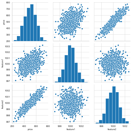
# df (obiettivo: predizione del price)
df = pd.read_csv('fake_reg.csv')
df.head()
| price | feature1 | feature2 | |
|---|---|---|---|
| 0 | 461.527929 | 999.787558 | 999.766096 |
| 1 | 548.130011 | 998.861615 | 1001.042403 |
| 2 | 410.297162 | 1000.070267 | 998.844015 |
| 3 | 540.382220 | 999.952251 | 1000.440940 |
| 4 | 546.024553 | 1000.446011 | 1000.338531 |
1
2
3
# pairplot
sns.set_style('whitegrid')
sns.pairplot(df, palette='red')
1
<seaborn.axisgrid.PairGrid at 0x2722a98fec8>
1
2
3
# X e y come np array
X = df[['feature1','feature2']].values
y = df['price'].values
1
2
3
4
# train test
X_train, X_test, y_train, y_test = train_test_split(X, y, test_size=0.3, random_state=42)
print(X_train.shape)
print(X_test.shape)
1
2
(700, 2)
(300, 2)
1
2
# min max scaling -- help
help(MinMaxScaler)
1
2
3
4
5
6
7
8
9
10
11
12
13
14
15
16
17
18
19
20
21
Help on class MinMaxScaler in module sklearn.preprocessing._data:

class MinMaxScaler(sklearn.base.TransformerMixin, sklearn.base.BaseEstimator)
 |  MinMaxScaler(feature_range=(0, 1), *, copy=True)
 |
 |  Transform features by scaling each feature to a given range.
 |
 |  This estimator scales and translates each feature individually such
 |  that it is in the given range on the training set, e.g. between
 |  zero and one.
 |
 |  The transformation is given by::
 |
 |      X_std = (X - X.min(axis=0)) / (X.max(axis=0) - X.min(axis=0))
 |      X_scaled = X_std * (max - min) + min
 |
 |  where min, max = feature_range.
 |
 |  This transformation is often used as an alternative to zero mean,
 |  unit variance scaling.
 |  ...
1
2
3
4
5
# min max scaling
scaler = MinMaxScaler()
scaler.fit(X_train)
X_train = scaler.transform(X_train)
X_test = scaler.transform(X_test)
1
2
print('Train Min-Max: ', X_train.min(), X_train.max())
print('Test Min-Max: ', X_test.min(), X_test.max())
1
2
Train Min-Max:  0.0 1.0
Test Min-Max:  -0.014108392024496652 1.0186515935232023
Choosing an optimizer and loss
Seguono i principali problemi supervisionati con Keras:
- Multi-class classification problem
1
# model.compile(optimizer='rmsprop', loss='categorical_crossentropy', metrics=['accuracy']) - Binary classification problem
1
# model.compile(optimizer='rmsprop', loss='binary_crossentropy', metrics=['accuracy']) - Mean squared error regression problem
1
# model.compile(optimizer='rmsprop', loss='mse')
1
2
3
4
5
# set seed per ridurre la non determinatezza del fit via GPU
os.environ['PYTHONHASHSEED'] = '13111990'
np.random.seed(13)
rn.seed(11)
tf.random.set_seed(1990)
1
2
3
4
5
6
7
8
9
# define model multiple line (si possono passare i Dense anche dentro il Sequential come lista)
model = Sequential()
model.add(Dense(units=4,activation='relu')) # units sono i nodi
model.add(Dense(units=4,activation='relu'))
model.add(Dense(units=4,activation='relu'))
model.add(Dense(units=1)) # final layer (vogliamo solo il price)

model.compile(optimizer='rmsprop',loss='mse')
# nb. questo passo mangia la GPU
Training
Descrizione parametri principali in Keras:
- Sample: one element of a dataset.
- Example: one image is a sample in a convolutional network
- Example: one audio file is a sample for a speech recognition model
- Batch: a set of N samples. The samples in a batch are processed independently, in parallel. If training, a batch results in only one update to the model.A batch generally approximates the distribution of the input data better than a single input. The larger the batch, the better the approximation; however, it is also true that the batch will take longer to process and will still result in only one update. For inference (evaluate/predict), it is recommended to pick a batch size that is as large as you can afford without going out of memory (since larger batches will usually result in faster evaluation/prediction).
- Epoch: an arbitrary cutoff, generally defined as “one pass over the entire dataset”, used to separate training into distinct phases, which is useful for logging and periodic evaluation.
- When using validation_data or validation_split with the fit method of Keras models, evaluation will be run at the end of every epoch.
1
2
3
4
5
# set seed per ridurre la non determinatezza del fit via GPU
os.environ['PYTHONHASHSEED'] = '13111990'
np.random.seed(13)
rn.seed(11)
tf.random.set_seed(1990)
1
2
# training model
model.fit(X_train,y_train,epochs=250)
1
2
3
4
5
6
7
8
9
10
Train on 700 samples
Epoch 1/250
700/700 [==============================] - 1s 2ms/sample - loss: 256557.3441
Epoch 2/250
700/700 [==============================] - 0s 73us/sample - loss: 256365.9997
...
Epoch 250/250
700/700 [==============================] - 0s 58us/sample - loss: 24.1132

<tensorflow.python.keras.callbacks.History at 0x27236051688>
Evaluation
1
2
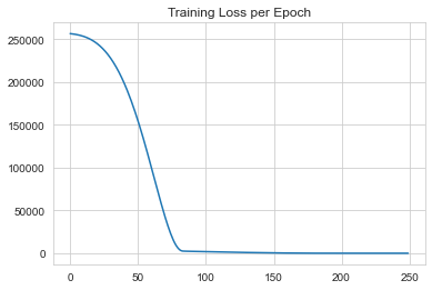
# loss trend
loss = model.history.history['loss']
1
2
3
# plot loss trend
sns.lineplot(x=range(len(loss)),y=loss)
plt.title("Training Loss per Epoch")
1
Text(0.5, 1.0, 'Training Loss per Epoch')
1
2
3
4
5
# Loss (in questo caso MSE)
training_score = model.evaluate(X_train,y_train,verbose=0)
test_score = model.evaluate(X_test,y_test,verbose=0)
print('training Score:', training_score)
print('test Score:', test_score)
1
2
training Score: 23.728277675083707
test Score: 25.146427205403647
1
2
# predictions
test_predictions = model.predict(X_test)
1
2
# previsti
test_predictions = pd.Series(test_predictions.reshape(300,))
1
2
3
# osservati
pred_df = pd.DataFrame(y_test,columns=['Test Y'])
pred_df.head()
| Test Y | |
|---|---|
| 0 | 402.296319 |
| 1 | 624.156198 |
| 2 | 582.455066 |
| 3 | 578.588606 |
| 4 | 371.224104 |
1
2
3
4
# previsti e osservati
pred_df = pd.concat([pred_df,test_predictions],axis=1)
pred_df.columns = ['Test Y','Model Predictions']
pred_df.head()
| Test Y | Model Predictions | |
|---|---|---|
| 0 | 402.296319 | 405.533844 |
| 1 | 624.156198 | 623.994934 |
| 2 | 582.455066 | 592.561340 |
| 3 | 578.588606 | 572.621155 |
| 4 | 371.224104 | 366.802795 |
1
2
3
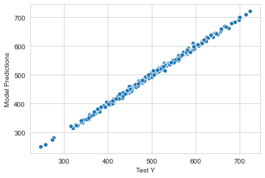
# scatter predict vs observed
sns.set_style('whitegrid')
sns.scatterplot(x='Test Y',y='Model Predictions',data=pred_df)
1
<matplotlib.axes._subplots.AxesSubplot at 0x27238970d08>
1
2
3
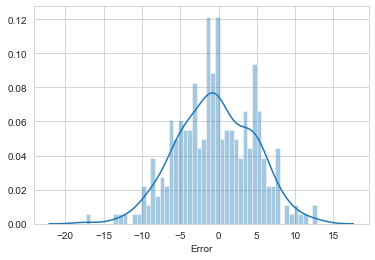
# distribution errors
pred_df['Error'] = pred_df['Test Y'] - pred_df['Model Predictions']
sns.distplot(pred_df['Error'],bins=50)
1
<matplotlib.axes._subplots.AxesSubplot at 0x27235ddbd88>
1
2
3
4
5
# metrics
print('MAE:',mean_absolute_error(pred_df['Test Y'],pred_df['Model Predictions']))
print('MSE:',mean_squared_error(pred_df['Test Y'],pred_df['Model Predictions']))
print('MSE (from model.evaluate):',test_score)
print('RMSE:',test_score**0.5)
1
2
3
4
MAE: 4.023428708666904
MSE: 25.14642937056938
MSE (from model.evaluate): 25.146427205403647
RMSE: 5.014621342175663
1
2
# Il MAE di circa 4, un errore di meno dell'1% della media
df['price'].describe()
1
2
3
4
5
6
7
8
9
count    1000.000000
mean      498.673029
std        93.785431
min       223.346793
25%       433.025732
50%       502.382117
75%       564.921588
max       774.407854
Name: price, dtype: float64
New observation to predict
1
2
3
4
5
6
# [[Feature1, Feature2]]
new_gem = [[998,1000]]
# scaling
new_gem = scaler.transform(new_gem)
# predict
print(model.predict(new_gem))
1
[[419.92566]]
Saving model
1
2
# working directory
os.getcwd()
1
'F:\\Python\\Course 001'
1
2
# save
model.save('Keras_Neural_Network_Example.h5')  # creates a HDF5 file
1
2
# load
later_model = load_model(r'F:\GitHub\AlbGri.github.io\assets\files\Python\Course 001\Keras_Neural_Network_Example.h5')
1
WARNING:tensorflow:Sequential models without an `input_shape` passed to the first layer cannot reload their optimizer state. As a result, your model isstarting with a freshly initialized optimizer.
1
2
# prediction with loaded model
print(later_model.predict(new_gem))
1
[[420.05133]]
House Sales in King County
Kaggle: Predict house price using regression
1
2
3
4
5
6
7
8
9
10
11
12
# lib
import pandas as pd
import numpy as np
import matplotlib.pyplot as plt
import seaborn as sns

from sklearn.model_selection import train_test_split
from sklearn.preprocessing import MinMaxScaler
from tensorflow.keras.models import Sequential
from tensorflow.keras.layers import Dense, Activation
from tensorflow.keras.optimizers import Adam
from sklearn.metrics import mean_squared_error,mean_absolute_error,explained_variance_score
1
2
3
# df
df = pd.read_csv('/kc_house_data.csv')
df.head()
| id | date | price | bedrooms | bathrooms | sqft_living | sqft_lot | floors | waterfront | view | ... | grade | sqft_above | sqft_basement | yr_built | yr_renovated | zipcode | lat | long | sqft_living15 | sqft_lot15 | |
|---|---|---|---|---|---|---|---|---|---|---|---|---|---|---|---|---|---|---|---|---|---|
| 0 | 7129300520 | 10/13/2014 | 221900.0 | 3 | 1.00 | 1180 | 5650 | 1.0 | 0 | 0 | ... | 7 | 1180 | 0 | 1955 | 0 | 98178 | 47.5112 | -122.257 | 1340 | 5650 |
| 1 | 6414100192 | 12/9/2014 | 538000.0 | 3 | 2.25 | 2570 | 7242 | 2.0 | 0 | 0 | ... | 7 | 2170 | 400 | 1951 | 1991 | 98125 | 47.7210 | -122.319 | 1690 | 7639 |
| 2 | 5631500400 | 2/25/2015 | 180000.0 | 2 | 1.00 | 770 | 10000 | 1.0 | 0 | 0 | ... | 6 | 770 | 0 | 1933 | 0 | 98028 | 47.7379 | -122.233 | 2720 | 8062 |
| 3 | 2487200875 | 12/9/2014 | 604000.0 | 4 | 3.00 | 1960 | 5000 | 1.0 | 0 | 0 | ... | 7 | 1050 | 910 | 1965 | 0 | 98136 | 47.5208 | -122.393 | 1360 | 5000 |
| 4 | 1954400510 | 2/18/2015 | 510000.0 | 3 | 2.00 | 1680 | 8080 | 1.0 | 0 | 0 | ... | 8 | 1680 | 0 | 1987 | 0 | 98074 | 47.6168 | -122.045 | 1800 | 7503 |
5 rows × 21 columns
1
df.info()
1
2
3
4
5
6
7
8
9
10
11
12
13
14
15
16
17
18
19
20
21
22
23
24
25
26
27
28
<class 'pandas.core.frame.DataFrame'>
RangeIndex: 21597 entries, 0 to 21596
Data columns (total 21 columns):
 #   Column         Non-Null Count  Dtype
---  ------         --------------  -----
 0   id             21597 non-null  int64
 1   date           21597 non-null  object
 2   price          21597 non-null  float64
 3   bedrooms       21597 non-null  int64
 4   bathrooms      21597 non-null  float64
 5   sqft_living    21597 non-null  int64
 6   sqft_lot       21597 non-null  int64
 7   floors         21597 non-null  float64
 8   waterfront     21597 non-null  int64
 9   view           21597 non-null  int64
 10  condition      21597 non-null  int64
 11  grade          21597 non-null  int64
 12  sqft_above     21597 non-null  int64
 13  sqft_basement  21597 non-null  int64
 14  yr_built       21597 non-null  int64
 15  yr_renovated   21597 non-null  int64
 16  zipcode        21597 non-null  int64
 17  lat            21597 non-null  float64
 18  long           21597 non-null  float64
 19  sqft_living15  21597 non-null  int64
 20  sqft_lot15     21597 non-null  int64
dtypes: float64(5), int64(15), object(1)
memory usage: 3.5+ MB
1
2
# converto id a stringa (così non la escludiamo tra le misure di sintesi)
df['id'] = df['id'].apply(str)
EDA
1
2
# check missing
df.isnull().sum().sum()
1
0
1
2
# per mostrare i separatori delle migliaia come punti e decimali come virgola
dot_sep = lambda x: format(round(x,2) if abs(x) < 1 else round(x,1) if abs(x) < 10 else int(x), ',').replace(",", "X").replace(".", ",").replace("X", ".")
1
2
3
4
# describe, potrei usare il .transpose, ma preferico così e miglioro i decimali
df.describe(percentiles=[0.25,0.5,0.75,0.999]).applymap(dot_sep)
# df.describe(percentiles=[0.25,0.5,0.75,0.999]).style.format("{:.1f}")
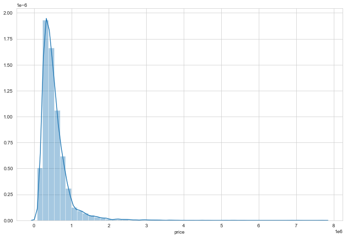
# sono presenti forti outliers
| price | bedrooms | bathrooms | sqft_living | sqft_lot | floors | waterfront | view | condition | grade | sqft_above | sqft_basement | yr_built | yr_renovated | lat | long | sqft_living15 | sqft_lot15 | month | year | |
|---|---|---|---|---|---|---|---|---|---|---|---|---|---|---|---|---|---|---|---|---|
| count | 21.597 | 21.597 | 21.597 | 21.597 | 21.597 | 21.597 | 21.597 | 21.597 | 21.597 | 21.597 | 21.597 | 21.597 | 21.597 | 21.597 | 21.597 | 21.597 | 21.597 | 21.597 | 21.597 | 21.597 |
| mean | 540.296 | 3,4 | 2,1 | 2.080 | 15.099 | 1,5 | 0,01 | 0,23 | 3,4 | 7,7 | 1.788 | 291 | 1.970 | 84 | 47 | -122 | 1.986 | 12.758 | 6,6 | 2.014 |
| std | 367.368 | 0,93 | 0,77 | 918 | 41.412 | 0,54 | 0,09 | 0,77 | 0,65 | 1,2 | 827 | 442 | 29 | 401 | 0,14 | 0,14 | 685 | 27.274 | 3,1 | 0,47 |
| min | 78.000 | 1,0 | 0,5 | 370 | 520 | 1,0 | 0,0 | 0,0 | 1,0 | 3,0 | 370 | 0,0 | 1.900 | 0,0 | 47 | -122 | 399 | 651 | 1,0 | 2.014 |
| 25% | 322.000 | 3,0 | 1,8 | 1.430 | 5.040 | 1,0 | 0,0 | 0,0 | 3,0 | 7,0 | 1.190 | 0,0 | 1.951 | 0,0 | 47 | -122 | 1.490 | 5.100 | 4,0 | 2.014 |
| 50% | 450.000 | 3,0 | 2,2 | 1.910 | 7.618 | 1,5 | 0,0 | 0,0 | 3,0 | 7,0 | 1.560 | 0,0 | 1.975 | 0,0 | 47 | -122 | 1.840 | 7.620 | 6,0 | 2.014 |
| 75% | 645.000 | 4,0 | 2,5 | 2.550 | 10.685 | 2,0 | 0,0 | 0,0 | 4,0 | 8,0 | 2.210 | 560 | 1.997 | 0,0 | 47 | -122 | 2.360 | 10.083 | 9,0 | 2.015 |
| 99.9% | 3.480.600 | 8,0 | 5,5 | 7.290 | 495.972 | 3,0 | 1,0 | 4,0 | 5,0 | 12 | 6.114 | 2.372 | 2.015 | 2.014 | 47 | -121 | 5.012 | 303.191 | 12 | 2.015 |
| max | 7.700.000 | 33 | 8,0 | 13.540 | 1.651.359 | 3,5 | 1,0 | 4,0 | 5,0 | 13 | 9.410 | 4.820 | 2.015 | 2.015 | 47 | -121 | 6.210 | 871.200 | 12 | 2.015 |
1
2
3
4
# distribuzione (continua) del price
sns.set_style('whitegrid')
plt.figure(figsize=(12,8))
sns.distplot(df['price'])
1
<matplotlib.axes._subplots.AxesSubplot at 0x18ba0584148>
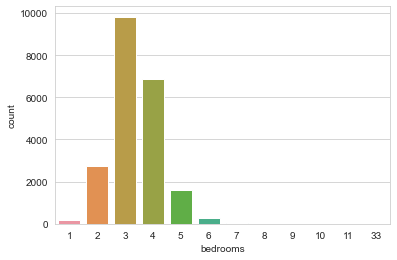
1
2
# distribuzione (discreta) bedrooms
sns.countplot(df['bedrooms'])
1
<matplotlib.axes._subplots.AxesSubplot at 0x18ba2b8e148>
1
2
# correlazioni con target
df.corr()['price'].sort_values()[-10:]
1
2
3
4
5
6
7
8
9
10
11
lat 0.306692
bedrooms 0.308787
sqft_basement 0.323799
view 0.397370
bathrooms 0.525906
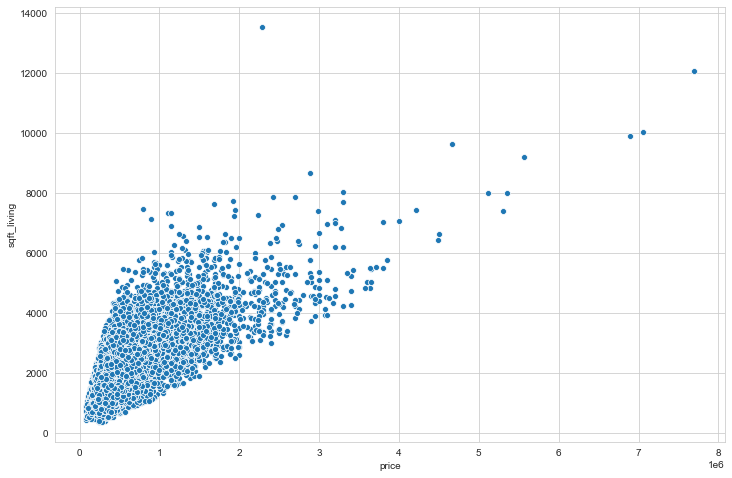
sqft_living15 0.585241
sqft_above 0.605368
grade 0.667951
sqft_living 0.701917
price 1.000000
Name: price, dtype: float64
1
2
3
# scatterplot price e sqft_living
plt.figure(figsize=(12,8))
sns.scatterplot(x='price',y='sqft_living',data=df)
1
<matplotlib.axes._subplots.AxesSubplot at 0x18ba1a2c0c8>
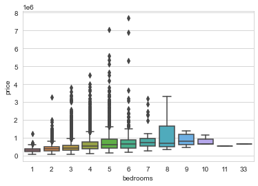
1
2
# boxplot bedrooms e price
sns.boxplot(x='bedrooms',y='price',data=df)
1
<matplotlib.axes._subplots.AxesSubplot at 0x18ba29eb148>
1
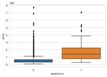
2
# boxplot waterfront e price
sns.boxplot(x='waterfront',y='price',data=df)
1
<matplotlib.axes._subplots.AxesSubplot at 0x18ba4e746c8>
Geographical Properties
1
2
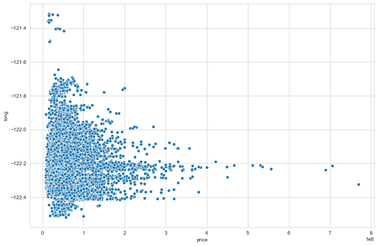
3
# il prezzo varia in funzione della longitudine?
plt.figure(figsize=(12,8))
sns.scatterplot(x='price',y='long',data=df)
1
<matplotlib.axes._subplots.AxesSubplot at 0x18ba2eda608>
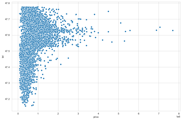
1
2
3
# il prezzo varia in funzione della latitudine?
plt.figure(figsize=(12,8))
sns.scatterplot(x='price',y='lat',data=df)
1
<matplotlib.axes._subplots.AxesSubplot at 0x18ba2f71108>
1
2
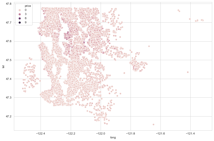
3
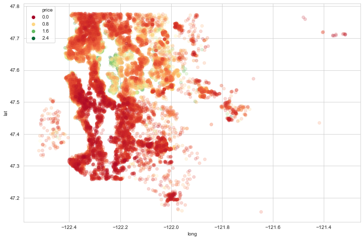
4
# plot latitudine e longitudine (King County)
plt.figure(figsize=(12,8))
sns.scatterplot(x='long',y='lat',data=df,hue='price')
# il colore non è distribuito bene perché ci sono forti outliers che spingono la distribuzione verso il basso
1
<matplotlib.axes._subplots.AxesSubplot at 0x18ba2ebc508>
1
2
# top 10 outliers per price
df.select_dtypes(include=np.number).sort_values('price',ascending=False).head(10).applymap(dot_sep)
| price | bedrooms | bathrooms | sqft_living | sqft_lot | floors | waterfront | view | condition | grade | sqft_above | sqft_basement | yr_built | yr_renovated | lat | long | sqft_living15 | sqft_lot15 | month | year | |
|---|---|---|---|---|---|---|---|---|---|---|---|---|---|---|---|---|---|---|---|---|
| 7245 | 7.700.000 | 6 | 8,0 | 12.050 | 27.600 | 2,5 | 0 | 3 | 4 | 13 | 8.570 | 3.480 | 1.910 | 1.987 | 47 | -122 | 3.940 | 8.800 | 10 | 2.014 |
| 3910 | 7.060.000 | 5 | 4,5 | 10.040 | 37.325 | 2,0 | 1 | 2 | 3 | 11 | 7.680 | 2.360 | 1.940 | 2.001 | 47 | -122 | 3.930 | 25.449 | 6 | 2.014 |
| 9245 | 6.890.000 | 6 | 7,8 | 9.890 | 31.374 | 2,0 | 0 | 4 | 3 | 13 | 8.860 | 1.030 | 2.001 | 0 | 47 | -122 | 4.540 | 42.730 | 9 | 2.014 |
| 4407 | 5.570.000 | 5 | 5,8 | 9.200 | 35.069 | 2,0 | 0 | 0 | 3 | 13 | 6.200 | 3.000 | 2.001 | 0 | 47 | -122 | 3.560 | 24.345 | 8 | 2.014 |
| 1446 | 5.350.000 | 5 | 5,0 | 8.000 | 23.985 | 2,0 | 0 | 4 | 3 | 12 | 6.720 | 1.280 | 2.009 | 0 | 47 | -122 | 4.600 | 21.750 | 4 | 2.015 |
| 1313 | 5.300.000 | 6 | 6,0 | 7.390 | 24.829 | 2,0 | 1 | 4 | 4 | 12 | 5.000 | 2.390 | 1.991 | 0 | 47 | -122 | 4.320 | 24.619 | 4 | 2.015 |
| 1162 | 5.110.000 | 5 | 5,2 | 8.010 | 45.517 | 2,0 | 1 | 4 | 3 | 12 | 5.990 | 2.020 | 1.999 | 0 | 47 | -122 | 3.430 | 26.788 | 10 | 2.014 |
| 8085 | 4.670.000 | 5 | 6,8 | 9.640 | 13.068 | 1,0 | 1 | 4 | 3 | 12 | 4.820 | 4.820 | 1.983 | 2.009 | 47 | -122 | 3.270 | 10.454 | 6 | 2.014 |
| 2624 | 4.500.000 | 5 | 5,5 | 6.640 | 40.014 | 2,0 | 1 | 4 | 3 | 12 | 6.350 | 290 | 2.004 | 0 | 47 | -122 | 3.030 | 23.408 | 8 | 2.014 |
| 8629 | 4.490.000 | 4 | 3,0 | 6.430 | 27.517 | 2,0 | 0 | 0 | 3 | 12 | 6.430 | 0 | 2.001 | 0 | 47 | -122 | 3.720 | 14.592 | 6 | 2.014 |
1
2
# escludo l'1% di coda del dataset, cioè 216 osservazioni
non_top_1_perc = df.sort_values('price',ascending=False).iloc[216:]
1
2
3
4
5
# plot latitudine e longitudine senza l'1% di coda
plt.figure(figsize=(12,8))
sns.scatterplot(x='long',y='lat',
                data=non_top_1_perc,hue='price',
                palette='RdYlGn',edgecolor=None,alpha=0.2)
1
<matplotlib.axes._subplots.AxesSubplot at 0x18ba4fdd148>
Feature Engineering
1
2
# drop id
df = df.drop('id',axis=1)
1
2
3
4
5
6
7
# engineering date
# convertiamo da string a time così è più semplice estrarre le info
df['date_string'] = df['date']
df['date'] = pd.to_datetime(df['date_string'])
df['month'] = df['date'].apply(lambda x: x.month)
df['year'] = df['date'].apply(lambda x: x.year)
df[['date_string','date','month','year']].info()
1
2
3
4
5
6
7
8
9
10
11
<class 'pandas.core.frame.DataFrame'>
RangeIndex: 21597 entries, 0 to 21596
Data columns (total 4 columns):
 #   Column       Non-Null Count  Dtype
---  ------       --------------  -----
 0   date_string  21597 non-null  object
 1   date         21597 non-null  datetime64[ns]
 2   month        21597 non-null  int64
 3   year         21597 non-null  int64
dtypes: datetime64[ns](1), int64(2), object(1)
memory usage: 675.0+ KB
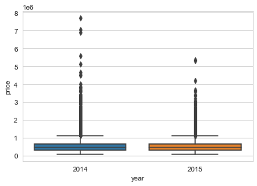
1
2
# boxplot anno price
sns.boxplot(x='year',y='price',data=df)
1
<matplotlib.axes._subplots.AxesSubplot at 0x18ba4e86308>
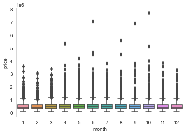
1
2
# boxplot mese price
sns.boxplot(x='month',y='price',data=df)
1
<matplotlib.axes._subplots.AxesSubplot at 0x18ba5505408>
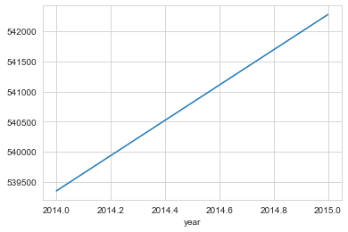
1
2
# andamento prezzo medio per mese
df.groupby('month').mean()['price'].plot()
1
<matplotlib.axes._subplots.AxesSubplot at 0x18ba197cac8>

1
2
# andamento prezzo medio per anno
df.groupby('year').mean()['price'].plot()
1
<matplotlib.axes._subplots.AxesSubplot at 0x18ba5090648>
1
2
3
# escludo le variabili con le date complete
df = df.drop(['date','date_string'],axis=1)
df.columns
1
2
3
4
5
Index(['price', 'bedrooms', 'bathrooms', 'sqft_living', 'sqft_lot', 'floors',
       'waterfront', 'view', 'condition', 'grade', 'sqft_above',
       'sqft_basement', 'yr_built', 'yr_renovated', 'zipcode', 'lat', 'long',
       'sqft_living15', 'sqft_lot15', 'month', 'year'],
      dtype='object')
1
2
3
4
# lo zip code va lavorato o escluso. lo escludiamo.
# se si include nel modello verrebbe considerato come numerico
# ci sono 70 zipcode diversi, quindi è un problema renderli dummy, si potrebbero raggruppare come zipcode più ricchi e meno ricchi, oppure fare raggruppamenti geografici come nord/centro/sud
df = df.drop('zipcode',axis=1)
1
2
3
# la maggior parte dei yr_renoveted sono 0, si potrebbe discretizzare come chi ha rinnovato e chi no.
# inoltre c'è una correlazione, più è recente e più sono i casi
df['yr_renovated'].value_counts()
1
2
3
4
5
6
7
8
9
10
11
12
0       20683
2014       91
2013       37
2003       36
2000       35
        ...
1934        1
1959        1
1951        1
1948        1
1944        1
Name: yr_renovated, Length: 70, dtype: int64
1
2
# la maggior parte dei sqft_basement sono 0, si potrebbe discretizzare come chi ha rinnovato e chi no
df['sqft_basement'].value_counts()
1
2
3
4
5
6
7
8
9
10
11
12
0       13110
600       221
700       218
500       214
800       206
        ...
792         1
2590        1
935         1
2390        1
248         1
Name: sqft_basement, Length: 306, dtype: int64
Models
1
2
3
# X e y
X = df.drop('price',axis=1)
y = df['price']
1
2
# train test
X_train, X_test, y_train, y_test = train_test_split(X,y,test_size=0.3,random_state=101)
1
2
3
4
5
6
# scaling Min Max
scaler = MinMaxScaler()
X_train = scaler.fit_transform(X_train) # attenzione il fit solo sul train
X_test = scaler.transform(X_test)
print(X_train.shape)
print(X_test.shape)
1
2
(15117, 19)
(6480, 19)
1
2
3
4
5
6
7
8
9
10
# definisco il modello
model = Sequential()

model.add(Dense(19,activation='relu'))
model.add(Dense(19,activation='relu'))
model.add(Dense(19,activation='relu'))
model.add(Dense(19,activation='relu'))
model.add(Dense(1))

model.compile(optimizer='adam',loss='mse')
1
2
3
4
5
# stimo il modello
model.fit(x=X_train,y=y_train.values,
          validation_data=(X_test,y_test.values),
          verbose=2,batch_size=128,epochs=400)
# il validation non viene utilizzato per il tuning solo per monitorare
1
2
3
4
5
6
7
8
9
Train on 15117 samples, validate on 6480 samples
Epoch 1/400
15117/15117 - 0s - loss: 96382199451.0191 - val_loss: 92658238633.4025
Epoch 2/400
...
Epoch 400/400
15117/15117 - 0s - loss: 29373463675.0805 - val_loss: 27157900968.1383

<tensorflow.python.keras.callbacks.History at 0x18bafce7548>
1
2
3
4
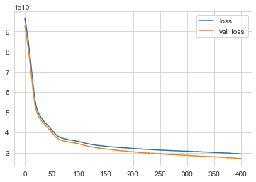
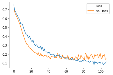
# andamento loss (mse)
losses = pd.DataFrame(model.history.history)
losses.plot()
# val_loss è sul test set, utile per capire se sto facendo overfit. non stiamo facendo overfit, potremmo continuare con le epochs.
1
<matplotlib.axes._subplots.AxesSubplot at 0x18bafd17f48>
1
2
# predictions
predictions = model.predict(X_test)
1
2
3
4
5
# metrics
print('MAE:',dot_sep(mean_absolute_error(y_test,predictions)))
print('MSE:',dot_sep(mean_squared_error(y_test,predictions)))
print('RMSE:',dot_sep(mean_squared_error(y_test,predictions)**0.5))
print('Explained Var Score:',dot_sep(explained_variance_score(y_test,predictions)))
1
2
3
4
MAE: 99.996
MSE: 27.157.901.022
RMSE: 164.796
Explained Var Score: 0,8
1
2
3
print('Media Price:',dot_sep(df['price'].mean()))
print('Mediana Price:',dot_sep(df['price'].median()))
# il MAE è di circa 100k, quindi un 20% della media
1
2
Media Price: 540.296
Mediana Price: 450.000
1
2
3
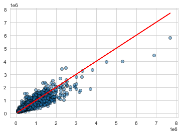
# plot osservate vs previste
plt.scatter(y_test,predictions,edgecolors='black',alpha=0.5)
plt.plot(y_test,y_test,'r')
1
[<matplotlib.lines.Line2D at 0x18bafcd3948>]
1
2
3
4
# distribuzione errori (devo formattarli uguali)
print(type(y_test))
print(type(predictions))
print(type(y_test.values.reshape(6480, 1)))
1
2
3
<class 'pandas.core.series.Series'>
<class 'numpy.ndarray'>
<class 'numpy.ndarray'>
1
2
3
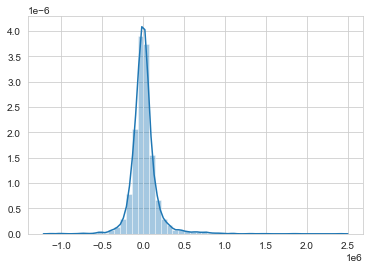
# distribuzione errori
errors = y_test.values.reshape(6480, 1) - predictions
sns.distplot(errors)
1
<matplotlib.axes._subplots.AxesSubplot at 0x18bb3093288>
Prediction on new observation
1
2
3
# esempio da prevedere
single_house = df.drop('price',axis=1).iloc[0]
single_house
1
2
3
4
5
6
7
8
9
10
11
12
13
14
15
16
17
18
19
20
bedrooms            3.0000
bathrooms           1.0000
sqft_living      1180.0000
sqft_lot         5650.0000
floors              1.0000
waterfront          0.0000
view                0.0000
condition           3.0000
grade               7.0000
sqft_above       1180.0000
sqft_basement       0.0000
yr_built         1955.0000
yr_renovated        0.0000
lat                47.5112
long             -122.2570
sqft_living15    1340.0000
sqft_lot15       5650.0000
month              10.0000
year             2014.0000
Name: 0, dtype: float64
1
2
3
# bisogna scalarlo e renderlo in formato vettore
single_house = scaler.transform(single_house.values.reshape(-1, 19))
single_house
1
2
3
4
array([[0.2       , 0.08      , 0.08376422, 0.00310751, 0.        ,
        0.        , 0.        , 0.5       , 0.4       , 0.10785619,
        0.        , 0.47826087, 0.        , 0.57149751, 0.21760797,
        0.16193426, 0.00582059, 0.81818182, 0.        ]])
1
2
# sappiamo qual è il target osservato
df.head(1)
| price | bedrooms | bathrooms | sqft_living | sqft_lot | floors | waterfront | view | condition | grade | sqft_above | sqft_basement | yr_built | yr_renovated | lat | long | sqft_living15 | sqft_lot15 | month | year | |
|---|---|---|---|---|---|---|---|---|---|---|---|---|---|---|---|---|---|---|---|---|
| 0 | 221900.0 | 3 | 1.0 | 1180 | 5650 | 1.0 | 0 | 0 | 3 | 7 | 1180 | 0 | 1955 | 0 | 47.5112 | -122.257 | 1340 | 5650 | 10 | 2014 |
1
2
3
# previsione
model.predict(single_house)
# si potrebbe migliorare il modello escludendo l'1% degli outliers e facendo più feature engineering
1
array([[294433.44]], dtype=float32)
Breast cancer Wisconsin
Keras Classification
1
2
3
4
5
6
7
8
9
10
11
12
13
14
15
16
17
18
# lib
import pandas as pd
import numpy as np

import seaborn as sns
import matplotlib.pyplot as plt

from sklearn.model_selection import train_test_split
from sklearn.preprocessing import MinMaxScaler
from sklearn.metrics import classification_report,confusion_matrix

import random as rn
import os

import tensorflow as tf
from tensorflow.keras.models import Sequential
from tensorflow.keras.layers import Dense, Activation,Dropout
from tensorflow.keras.callbacks import EarlyStopping
1
2
3
# df
df = pd.read_csv('cancer_classification.csv')
df.head()
| mean radius | mean texture | mean perimeter | mean area | mean smoothness | mean compactness | mean concavity | mean concave points | mean symmetry | mean fractal dimension | ... | worst texture | worst perimeter | worst area | worst smoothness | worst compactness | worst concavity | worst concave points | worst symmetry | worst fractal dimension | benign_0__mal_1 | |
|---|---|---|---|---|---|---|---|---|---|---|---|---|---|---|---|---|---|---|---|---|---|
| 0 | 17.99 | 10.38 | 122.80 | 1001.0 | 0.11840 | 0.27760 | 0.3001 | 0.14710 | 0.2419 | 0.07871 | ... | 17.33 | 184.60 | 2019.0 | 0.1622 | 0.6656 | 0.7119 | 0.2654 | 0.4601 | 0.11890 | 0 |
| 1 | 20.57 | 17.77 | 132.90 | 1326.0 | 0.08474 | 0.07864 | 0.0869 | 0.07017 | 0.1812 | 0.05667 | ... | 23.41 | 158.80 | 1956.0 | 0.1238 | 0.1866 | 0.2416 | 0.1860 | 0.2750 | 0.08902 | 0 |
| 2 | 19.69 | 21.25 | 130.00 | 1203.0 | 0.10960 | 0.15990 | 0.1974 | 0.12790 | 0.2069 | 0.05999 | ... | 25.53 | 152.50 | 1709.0 | 0.1444 | 0.4245 | 0.4504 | 0.2430 | 0.3613 | 0.08758 | 0 |
| 3 | 11.42 | 20.38 | 77.58 | 386.1 | 0.14250 | 0.28390 | 0.2414 | 0.10520 | 0.2597 | 0.09744 | ... | 26.50 | 98.87 | 567.7 | 0.2098 | 0.8663 | 0.6869 | 0.2575 | 0.6638 | 0.17300 | 0 |
| 4 | 20.29 | 14.34 | 135.10 | 1297.0 | 0.10030 | 0.13280 | 0.1980 | 0.10430 | 0.1809 | 0.05883 | ... | 16.67 | 152.20 | 1575.0 | 0.1374 | 0.2050 | 0.4000 | 0.1625 | 0.2364 | 0.07678 | 0 |
5 rows × 31 columns
1
2
# controllo missing
df.isnull().sum().sum()
1
0
1
2
# per mostrare i separatori delle migliaia come punti e decimali come virgola
dot_sep = lambda x: format(round(x,2) if abs(x) < 1 else round(x,1) if abs(x) < 10 else int(x), ',').replace(",", "X").replace(".", ",").replace("X", ".")
1
2
# describe, potrei usare il .transpose, ma preferico così e miglioro i decimali
df.describe(percentiles=[0.25,0.5,0.75,0.999]).applymap(dot_sep)
| mean radius | mean texture | mean perimeter | mean area | mean smoothness | mean compactness | mean concavity | mean concave points | mean symmetry | mean fractal dimension | ... | worst texture | worst perimeter | worst area | worst smoothness | worst compactness | worst concavity | worst concave points | worst symmetry | worst fractal dimension | benign_0__mal_1 | |
|---|---|---|---|---|---|---|---|---|---|---|---|---|---|---|---|---|---|---|---|---|---|
| count | 569 | 569 | 569 | 569 | 569 | 569 | 569 | 569 | 569 | 569 | ... | 569 | 569 | 569 | 569 | 569 | 569 | 569 | 569 | 569 | 569 |
| mean | 14 | 19 | 91 | 654 | 0,1 | 0,1 | 0,09 | 0,05 | 0,18 | 0,06 | ... | 25 | 107 | 880 | 0,13 | 0,25 | 0,27 | 0,11 | 0,29 | 0,08 | 0,63 |
| std | 3,5 | 4,3 | 24 | 351 | 0,01 | 0,05 | 0,08 | 0,04 | 0,03 | 0,01 | ... | 6,1 | 33 | 569 | 0,02 | 0,16 | 0,21 | 0,07 | 0,06 | 0,02 | 0,48 |
| min | 7,0 | 9,7 | 43 | 143 | 0,05 | 0,02 | 0,0 | 0,0 | 0,11 | 0,05 | ... | 12 | 50 | 185 | 0,07 | 0,03 | 0,0 | 0,0 | 0,16 | 0,06 | 0,0 |
| 25% | 11 | 16 | 75 | 420 | 0,09 | 0,06 | 0,03 | 0,02 | 0,16 | 0,06 | ... | 21 | 84 | 515 | 0,12 | 0,15 | 0,11 | 0,06 | 0,25 | 0,07 | 0,0 |
| 50% | 13 | 18 | 86 | 551 | 0,1 | 0,09 | 0,06 | 0,03 | 0,18 | 0,06 | ... | 25 | 97 | 686 | 0,13 | 0,21 | 0,23 | 0,1 | 0,28 | 0,08 | 1,0 |
| 75% | 15 | 21 | 104 | 782 | 0,11 | 0,13 | 0,13 | 0,07 | 0,2 | 0,07 | ... | 29 | 125 | 1.084 | 0,15 | 0,34 | 0,38 | 0,16 | 0,32 | 0,09 | 1,0 |
| 99.9% | 27 | 36 | 187 | 2.499 | 0,15 | 0,33 | 0,43 | 0,2 | 0,3 | 0,1 | ... | 48 | 238 | 3.787 | 0,22 | 0,99 | 1,2 | 0,29 | 0,61 | 0,19 | 1,0 |
| max | 28 | 39 | 188 | 2.501 | 0,16 | 0,35 | 0,43 | 0,2 | 0,3 | 0,1 | ... | 49 | 251 | 4.254 | 0,22 | 1,1 | 1,3 | 0,29 | 0,66 | 0,21 | 1,0 |
9 rows × 31 columns
1
2
3
4
5
6
7
8
9
10
11
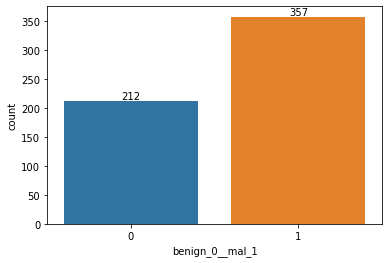
# verifichiamo la distribuzione target
ax = sns.countplot(x='benign_0__mal_1',data=df)
# non è troppo sbilanciato
# aggiungo le frequenze
for p in ax.patches:
height = p.get_height()
ax.text(p.get_x()+p.get_width()/2.,
height + 3,
'{:1.0f}'.format(height), # '{:1.2f}'.format(height/float(len(df)))
ha="center")
1
2
3
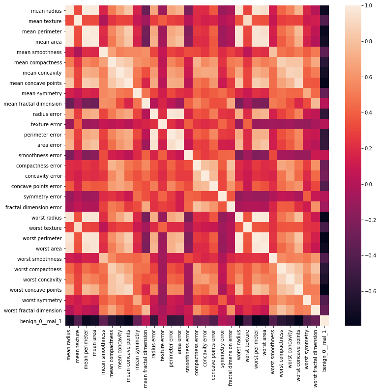
# heatmap
plt.figure(figsize=(12,12))
sns.heatmap(df.corr())
1
<matplotlib.axes._subplots.AxesSubplot at 0x26b02b93048>
1
2
# head e tail delle variabili più correlate con la target
pd.concat([df.corr()['benign_0__mal_1'].sort_values().head(),df.corr()['benign_0__mal_1'].sort_values().tail()])
1
2
3
4
5
6
7
8
9
10
11
worst concave points     -0.793566
worst perimeter          -0.782914
mean concave points      -0.776614
worst radius             -0.776454
mean perimeter           -0.742636
symmetry error            0.006522
texture error             0.008303
mean fractal dimension    0.012838
smoothness error          0.067016
benign_0__mal_1           1.000000
Name: benign_0__mal_1, dtype: float64
1
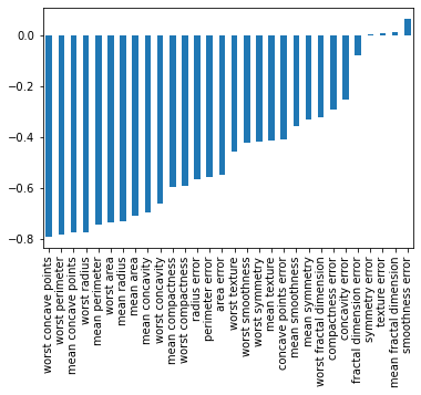
2
# correlate con la target (escludo la target)
df.corr()['benign_0__mal_1'][:-1].sort_values().plot(kind='bar')
1
<matplotlib.axes._subplots.AxesSubplot at 0x26b02bbbb88>
Model
1
2
3
# X e y (come numpy arrays)
X = df.drop('benign_0__mal_1',axis=1).values
y = df['benign_0__mal_1'].values
1
2
# train e test
X_train, X_test, y_train, y_test = train_test_split(X,y,test_size=0.25,random_state=101)
1
2
3
4
5
6
7
# scaling data
scaler = MinMaxScaler()
# scaler.fit(X_train) # stima i parametri
# X_train = scaler.transform(X_train) # applica i parametri
# X_test = scaler.transform(X_test)
X_train = scaler.fit_transform(X_train) # stima e applica i parametri in un solo comando
X_test = scaler.transform(X_test) # avevo erroneamente fatto il fit, non andava messo, si otterranno risultati leggermente diversi
1
2
3
4
5
# set seed per ridurre la non determinatezza del fit via GPU
os.environ['PYTHONHASHSEED'] = '13111990'
np.random.seed(13)
rn.seed(11)
tf.random.set_seed(1990)
1
2
3
4
5
6
7
8
# definizione struttura neural network per classificazione
model = Sequential()
# https://stats.stackexchange.com/questions/181/how-to-choose-the-number-of-hidden-layers-and-nodes-in-a-feedforward-neural-netw
model.add(Dense(units=30,activation='relu'))
model.add(Dense(units=15,activation='relu'))
model.add(Dense(units=1,activation='sigmoid'))
# For a binary classification problem
model.compile(loss='binary_crossentropy', optimizer='adam')
1
2
3
4
5
# set seed per ridurre la non determinatezza del fit via GPU
os.environ['PYTHONHASHSEED'] = '13111990'
np.random.seed(13)
rn.seed(11)
tf.random.set_seed(1990)
1
2
3
4
5
6
7
8
9
%%time
# stima modello con overfitting
# https://stats.stackexchange.com/questions/164876/tradeoff-batch-size-vs-number-of-iterations-to-train-a-neural-network
# https://datascience.stackexchange.com/questions/18414/are-there-any-rules-for-choosing-the-size-of-a-mini-batch
model.fit(x=X_train,
          y=y_train,
          epochs=600,
          validation_data=(X_test, y_test), verbose=0
          )
1
2
3
Wall time: 35.6 s

<tensorflow.python.keras.callbacks.History at 0x26b07120608>
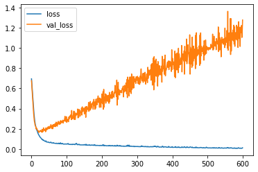
1
2
3
# loss crossentropy
model_loss = pd.DataFrame(model.history.history)
model_loss.plot()
1
<matplotlib.axes._subplots.AxesSubplot at 0x26b05f654c8>
Early Stopping
1
2
# 'Stop training when a monitored quantity has stopped improving'
help(EarlyStopping)
1
2
3
4
5
6
7
8
9
10
11
12
13
14
15
16
17
18
19
20
21
22
23
24
25
26
27
28
29
30
31
32
Help on class EarlyStopping in module tensorflow.python.keras.callbacks:

class EarlyStopping(Callback)
 |  EarlyStopping(monitor='val_loss', min_delta=0, patience=0, verbose=0, mode='auto', baseline=None, restore_best_weights=False)
 |
 |  Stop training when a monitored quantity has stopped improving.
 |
 |  Arguments:
 |      monitor: Quantity to be monitored.
 |      min_delta: Minimum change in the monitored quantity
 |          to qualify as an improvement, i.e. an absolute
 |          change of less than min_delta, will count as no
 |          improvement.
 |      patience: Number of epochs with no improvement
 |          after which training will be stopped.
 |      verbose: verbosity mode.
 |      mode: One of `{"auto", "min", "max"}`. In `min` mode,
 |          training will stop when the quantity
 |          monitored has stopped decreasing; in `max`
 |          mode it will stop when the quantity
 |          monitored has stopped increasing; in `auto`
 |          mode, the direction is automatically inferred
 |          from the name of the monitored quantity.
 |      baseline: Baseline value for the monitored quantity.
 |          Training will stop if the model doesn't show improvement over the
 |          baseline.
 |      restore_best_weights: Whether to restore model weights from
 |          the epoch with the best value of the monitored quantity.
 |          If False, the model weights obtained at the last step of
 |          training are used.
 |
 |  ...
1
2
3
4
5
# set seed per ridurre la non determinatezza del fit via GPU
os.environ['PYTHONHASHSEED'] = '13111990'
np.random.seed(13)
rn.seed(11)
tf.random.set_seed(1990)
1
2
3
4
5
6
# definizione struttura neural network per classificazione
model = Sequential()
model.add(Dense(units=30,activation='relu'))
model.add(Dense(units=15,activation='relu'))
model.add(Dense(units=1,activation='sigmoid'))
model.compile(loss='binary_crossentropy', optimizer='adam')
1
2
# definizione early stopping
early_stop = EarlyStopping(monitor='val_loss', mode='min', verbose=1, patience=25)
1
2
3
4
5
# set seed per ridurre la non determinatezza del fit via GPU
os.environ['PYTHONHASHSEED'] = '13111990'
np.random.seed(13)
rn.seed(11)
tf.random.set_seed(1990)
1
2
3
4
5
6
7
8
%%time
# stima modello con early stop per limitare overfitting
model.fit(x=X_train,
          y=y_train,
          epochs=600,
          validation_data=(X_test, y_test), verbose=0,
          callbacks=[early_stop]
          )
1
2
3
4
Epoch 00047: early stopping
Wall time: 3.06 s

<tensorflow.python.keras.callbacks.History at 0x26b08b5b2c8>
1
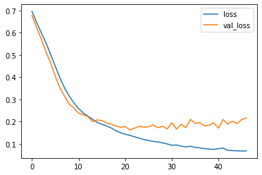
2
3
# loss crossentropy
model_loss = pd.DataFrame(model.history.history)
model_loss.plot()
1
<matplotlib.axes._subplots.AxesSubplot at 0x26b08f1bb48>
DropOut Layers
1
2
3
4
5
# set seed per ridurre la non determinatezza del fit via GPU
os.environ['PYTHONHASHSEED'] = '13111990'
np.random.seed(13)
rn.seed(11)
tf.random.set_seed(1990)
1
2
3
4
5
6
7
8
# definizione struttura neural network per classificazione
model = Sequential()
model.add(Dense(units=30,activation='relu'))
model.add(Dropout(0.5))
model.add(Dense(units=15,activation='relu'))
model.add(Dropout(0.5))
model.add(Dense(units=1,activation='sigmoid'))
model.compile(loss='binary_crossentropy', optimizer='adam')
1
2
3
4
5
# set seed per ridurre la non determinatezza del fit via GPU
os.environ['PYTHONHASHSEED'] = '13111990'
np.random.seed(13)
rn.seed(11)
tf.random.set_seed(1990)
1
2
3
4
5
6
7
8
%%time
# stima modello con early stop e dropout per limitare overfitting
model.fit(x=X_train,
          y=y_train,
          epochs=600,
          validation_data=(X_test, y_test), verbose=0,
          callbacks=[early_stop]
          )
1
2
3
4
Epoch 00107: early stopping
Wall time: 8.93 s

<tensorflow.python.keras.callbacks.History at 0x26b091d5b48>
1
2
3
# loss crossentropy
model_loss = pd.DataFrame(model.history.history)
model_loss.plot()
1
<matplotlib.axes._subplots.AxesSubplot at 0x26b0583fc08>
Metrics
1
2
# predictions
predictions = model.predict_classes(X_test)
1
2
3
4
5
# metrics
print('\nConfusion Matrix:')
print(confusion_matrix(y_test,predictions))
print('\nClassification metrics:')
print(classification_report(y_test,predictions))
1
2
3
4
5
6
7
8
9
10
11
12
13
Confusion Matrix:
[[54  1]
 [ 6 82]]

Classification metrics:
              precision    recall  f1-score   support

           0       0.90      0.98      0.94        55
           1       0.99      0.93      0.96        88

    accuracy                           0.95       143
   macro avg       0.94      0.96      0.95       143
weighted avg       0.95      0.95      0.95       143
LendingClub dataset
Kaggle: Predict default loans with classification
1
2
3
4
5
6
7
8
9
10
11
12
13
14
15
16
17
18
# lib
import pandas as pd
import numpy as np

import seaborn as sns
import matplotlib.pyplot as plt
%matplotlib inline

from sklearn.model_selection import train_test_split
from sklearn.preprocessing import MinMaxScaler
from sklearn.metrics import classification_report,confusion_matrix

import random as rn
import os

import tensorflow as tf
from tensorflow.keras.models import Sequential
from tensorflow.keras.layers import Dense, Activation, Dropout
1
2
3
# df
df = pd.read_csv('/lending_club_loan_two.csv')
df.info()
1
2
3
4
5
6
7
8
9
10
11
12
13
14
15
16
17
18
19
20
21
22
23
24
25
26
27
28
29
30
31
32
33
34
<class 'pandas.core.frame.DataFrame'>
RangeIndex: 396030 entries, 0 to 396029
Data columns (total 27 columns):
 #   Column                Non-Null Count   Dtype
---  ------                --------------   -----
 0   loan_amnt             396030 non-null  float64
 1   term                  396030 non-null  object
 2   int_rate              396030 non-null  float64
 3   installment           396030 non-null  float64
 4   grade                 396030 non-null  object
 5   sub_grade             396030 non-null  object
 6   emp_title             373103 non-null  object
 7   emp_length            377729 non-null  object
 8   home_ownership        396030 non-null  object
 9   annual_inc            396030 non-null  float64
 10  verification_status   396030 non-null  object
 11  issue_d               396030 non-null  object
 12  loan_status           396030 non-null  object
 13  purpose               396030 non-null  object
 14  title                 394275 non-null  object
 15  dti                   396030 non-null  float64
 16  earliest_cr_line      396030 non-null  object
 17  open_acc              396030 non-null  float64
 18  pub_rec               396030 non-null  float64
 19  revol_bal             396030 non-null  float64
 20  revol_util            395754 non-null  float64
 21  total_acc             396030 non-null  float64
 22  initial_list_status   396030 non-null  object
 23  application_type      396030 non-null  object
 24  mort_acc              358235 non-null  float64
 25  pub_rec_bankruptcies  395495 non-null  float64
 26  address               396030 non-null  object
dtypes: float64(12), object(15)
memory usage: 81.6+ MB
Step 1: EDA
1
2
3
4
5
6
7
8
9
10
11
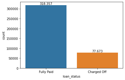
# verifichiamo la distribuzione target
ax = sns.countplot(x='loan_status',data=df)
# un po' sbilanciato, ci aspetteremo un'elevata accuracy ma precision e recall saranno quelle difficili
# aggiungo le frequenze
for p in ax.patches:
height = p.get_height()
ax.text(p.get_x()+p.get_width()/2.,
height+3000,
'{:,.0f}'.format(height).replace(",", "X").replace(".", ",").replace("X", "."), # '{:1.2f}'.format(height/float(len(df)))
ha="center")
1
2
3
4
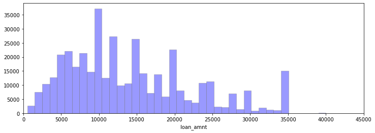
# histogram di loan_amnt
plt.figure(figsize=(12,4))
sns.distplot(df['loan_amnt'],kde=False,color='b',bins=40,hist_kws=dict(edgecolor='grey'))
plt.xlim(0,45000)
1
(0.0, 45000.0)
1
2
3
4
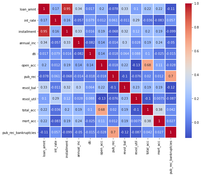
# heatmap
plt.figure(figsize=(10,8))
sns.heatmap(df.corr(),annot=True,cmap='coolwarm',linecolor='white',linewidths=1)
# plt.ylim(10, 0)
1
<matplotlib.axes._subplots.AxesSubplot at 0x2db149a6f88>
1
2
3
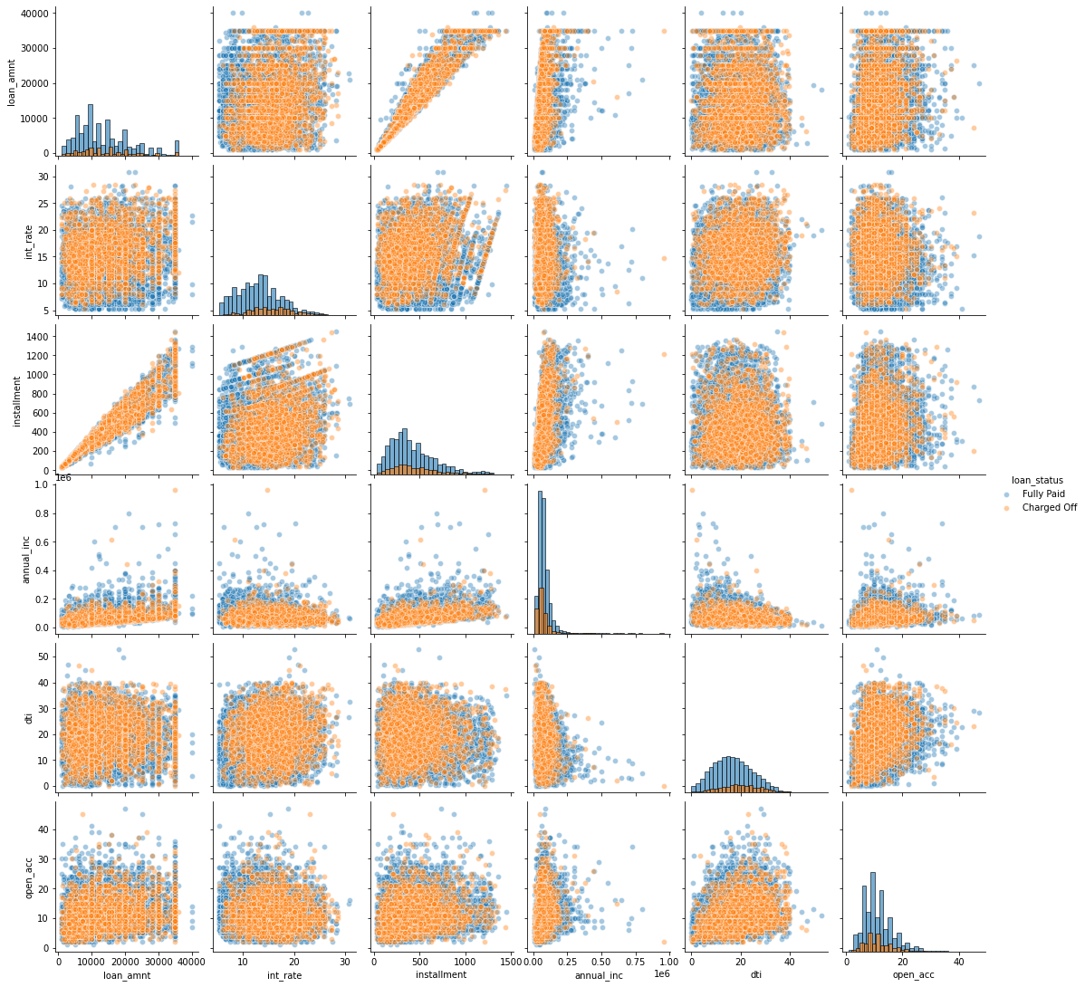
# mezzo-pairplot (parte 1)
df_pair1 = df[df.columns[0:18]].sample(n=10000, random_state=1311)
sns.pairplot(df_pair1,hue='loan_status',diag_kind='hist',diag_kws=dict(edgecolor='black',alpha=0.6,bins=30),plot_kws=dict(alpha=0.4))
1
<seaborn.axisgrid.PairGrid at 0x18e3e6a8cc8>
1
2
3
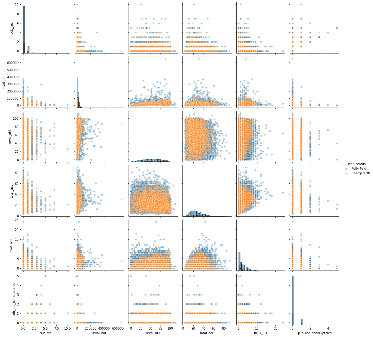
# mezzo-pairplot (parte 2)
df_pair2 = df.iloc[:, np.r_[12,18:27]].sample(n=10000, random_state=1311) # indexer
sns.pairplot(df_pair2,hue='loan_status',diag_kind='hist',diag_kws=dict(edgecolor='black',alpha=0.6,bins=30),plot_kws=dict(alpha=0.4))
1
<seaborn.axisgrid.PairGrid at 0x18e0a62d088>
1
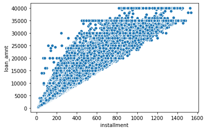
2
# scatterplot
sns.scatterplot(x='installment',y='loan_amnt',data=df)
1
<matplotlib.axes._subplots.AxesSubplot at 0x2db16fec1c8>
1
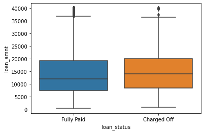
2
# boxplot loan_status e loan amount
sns.boxplot(x='loan_status',y='loan_amnt',data=df)
1
<matplotlib.axes._subplots.AxesSubplot at 0x2db177d3ac8>
1
2
3
4
5
# per mostrare i separatori delle migliaia come punti e decimali come virgola
dot_sep = lambda x: format(round(x,2) if abs(x) < 1 else round(x,1) if abs(x) < 10 else int(x), ',').replace(",", "X").replace(".", ",").replace("X", ".")

# loan amount by loan status
df.groupby('loan_status')['loan_amnt'].describe().applymap(dot_sep)
| count | mean | std | min | 25% | 50% | 75% | max | |
|---|---|---|---|---|---|---|---|---|
| loan_status | ||||||||
| Charged Off | 77.673 | 15.126 | 8.505 | 1.000 | 8.525 | 14.000 | 20.000 | 40.000 |
| Fully Paid | 318.357 | 13.866 | 8.302 | 500 | 7.500 | 12.000 | 19.225 | 40.000 |
1
2
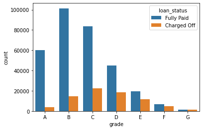
# countplot per grade stratificato per target
sns.countplot(x='grade',hue='loan_status',data=df,order=sorted(df['grade'].unique()))
1
<matplotlib.axes._subplots.AxesSubplot at 0x2a843721688>
1
2
3
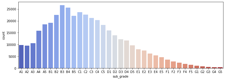
# countplot per subgrade
plt.figure(figsize=(12,4))
sns.countplot(x='sub_grade',data=df,order=sorted(df['sub_grade'].unique()),palette='coolwarm')
1
<matplotlib.axes._subplots.AxesSubplot at 0x2db14a6f548>
1
2
3
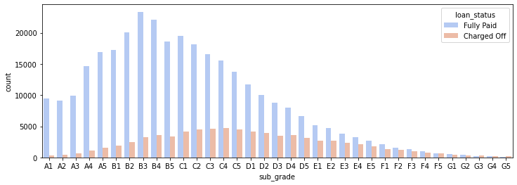
# countplot per subgrade stratificato per target
plt.figure(figsize=(12,4))
sns.countplot(x='sub_grade',data=df,order=sorted(df['sub_grade'].unique()),palette='coolwarm',hue='loan_status')
1
<matplotlib.axes._subplots.AxesSubplot at 0x2db16a31888>
1
2
3
4
5
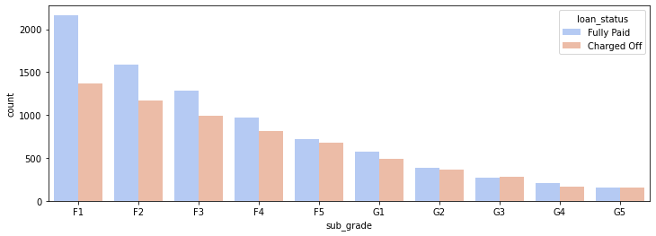
# countplot per subgrade (F e G) stratificato per target
plt.figure(figsize=(12,4))
df_FG = df[(df['grade']=='G') | (df['grade']=='F')]
# df_FG = df[df['sub_grade'].apply(lambda x: x[0] in ['G','F'])]
sns.countplot(x='sub_grade',data=df_FG,order=sorted(df_FG['sub_grade'].unique()),palette='coolwarm',hue='loan_status')
1
<matplotlib.axes._subplots.AxesSubplot at 0x2db1782ed48>
1
2
3
4
5
6
7
8
# il method map è il più veloce per la rimappatura di una variabile
mapping_dict = {'Fully Paid': 1, 'Charged Off': 0}
df['loan_status'].map(mapping_dict).value_counts() # se il mapping non è esaustivo invece dei NaN si può dare il valore originale con il metodo .fillna(df['loan_status'])

# Risultati identici ma meno performanti:
# df['loan_status'].replace(mapping_dict).value_counts()
# df.replace({'loan_status': mapping_dict})['loan_status'].value_counts() # così devo specificare la colonna e deve agire su tutto il df
# df['loan_status'].replace(to_replace=['Fully Paid', 'Charged Off'], value=[1, 0]).value_counts()
1
2
3
1    318357
0     77673
Name: loan_status, dtype: int64
1
2
3
4
5
6
# creo dummy/dicotomizzo la target loan status
df['loan_repaid'] = df['loan_status'].map({'Fully Paid':1,'Charged Off':0})
print(df.shape)
# tabella di contingenza
df.groupby(["loan_repaid", "loan_status"]).size().reset_index(name="Frequenza")
# pd.crosstab(df['loan_repaid'],df['loan_status'])
1
(396030, 28)
| loan_repaid | loan_status | Frequenza | |
|---|---|---|---|
| 0 | 0 | Charged Off | 77673 |
| 1 | 1 | Fully Paid | 318357 |
1
2
3
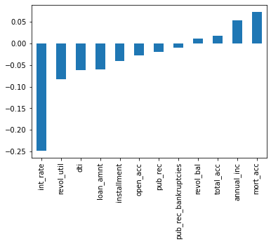
# correlazione target con le altre variabili numeriche
df.corr()['loan_repaid'][:-1].sort_values().plot(kind='bar')
# df.corr()['loan_repaid'].sort_values().drop('loan_repaid').plot(kind='bar')
1
<matplotlib.axes._subplots.AxesSubplot at 0x18e17784e48>
Step 2: Data Preprocessing
Section Goals: Remove or fill any missing data. Remove unnecessary or repetitive features. Convert categorical string features to dummy variables.
1
2
# df numero record
len(df)
1
396030
1
2
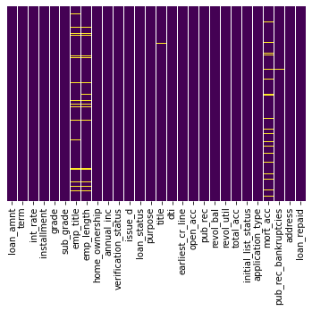
# missing data
sns.heatmap(df.isnull(),yticklabels=False,cbar=False,cmap='viridis')
1
<matplotlib.axes._subplots.AxesSubplot at 0x2db17a29148>
1
2
3
4
5
6
7
# missing data count
missing_counts = pd.concat(
[df.isnull().sum()[df.isnull().sum()>0].apply(dot_sep),
(df.isnull().sum()[df.isnull().sum()>0]/len(df)*100).apply(dot_sep)],
axis=1)
missing_counts.columns = ['Freq', 'Freq %']
missing_counts
| Freq | Freq % | |
|---|---|---|
| emp_title | 22.927 | 5,8 |
| emp_length | 18.301 | 4,6 |
| title | 1.755 | 0,44 |
| revol_util | 276 | 0,07 |
| mort_acc | 37.795 | 9,5 |
| pub_rec_bankruptcies | 535 | 0,14 |
1
2
3
4
5
6
# employement job titles univoci
print(df['emp_title'].value_counts())
print('\nUnivoci:',dot_sep(df['emp_title'].nunique()))
# troppe per creare dummy, la rimuovo ma si potrebbero raggruppare
df.drop('emp_title',inplace=True,axis=1)
print(df.shape)
1
2
3
4
5
6
7
8
9
10
11
12
13
14
15
Teacher 4389
Manager 4250
Registered Nurse 1856
RN 1846
Supervisor 1830
...
Annunciation 1
Atos Inc 1
chevy parts maneger 1
Architectural Intern 1
GroupSystems Corporation 1
Name: emp_title, Length: 173105, dtype: int64
Univoci: 173.105
(396030, 27)
1
2
3
4
# sorted(df['emp_length'].dropna().unique())
emp_length_order = ['Missing','< 1 year', '1 year', '2 years', '3 years',
'4 years', '5 years', '6 years', '7 years',
'8 years', '9 years', '10+ years']
1
2
3
4
5
6
7
8
9
10
11
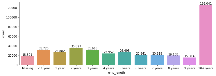
# countplot emp_length
plt.figure(figsize=(12,4))
ax = sns.countplot(x='emp_length',data=df[['emp_length']].fillna('Missing'),order=emp_length_order)
# aggiungo le frequenze
for p in ax.patches:
height = p.get_height()
ax.text(p.get_x()+p.get_width()/2.,
height + 1000,
'{:,.0f}'.format(height).replace(",", "X").replace(".", ",").replace("X", "."),
ha="center")
1
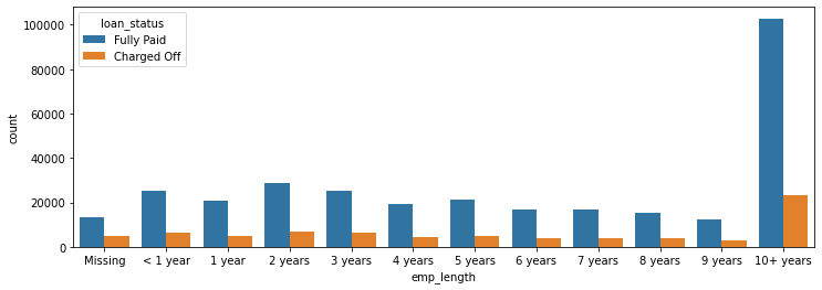
2
3
# countplot emp_length
plt.figure(figsize=(12,4))
sns.countplot(x='emp_length',data=df[['emp_length','loan_status']].fillna('Missing'),order=emp_length_order, hue='loan_status')
1
<matplotlib.axes._subplots.AxesSubplot at 0x2db203a15c8>
1
2
3
4
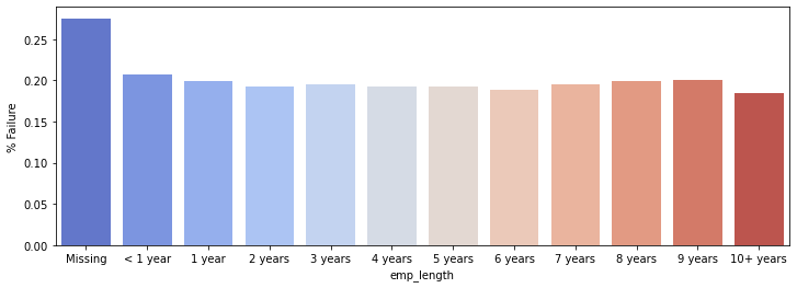
# tasso di insucesso per ogni emp_length
# emp_len = df[df['loan_status']=="Charged Off"].groupby("emp_length").count()['loan_status']/df.groupby("emp_length").count()['loan_status']
emp_len = pd.DataFrame(df[['emp_length','loan_status']].fillna('Missing').groupby(['emp_length','loan_status']).size().groupby(level=0).apply(lambda x: x / x.sum()).xs('Charged Off',level='loan_status'),columns=['% Failure']).reset_index()
emp_len
| emp_length | % Failure | |
|---|---|---|
| 0 | 1 year | 0.199135 |
| 1 | 10+ years | 0.184186 |
| 2 | 2 years | 0.193262 |
| 3 | 3 years | 0.195231 |
| 4 | 4 years | 0.192385 |
| 5 | 5 years | 0.192187 |
| 6 | 6 years | 0.189194 |
| 7 | 7 years | 0.194774 |
| 8 | 8 years | 0.199760 |
| 9 | 9 years | 0.200470 |
| 10 | < 1 year | 0.206872 |
| 11 | Missing | 0.275286 |
1
2
3
4
5
6
7
# barplot tasso
plt.figure(figsize=(12,4))
# emp_len.plot(kind='bar')
sns.barplot(x='emp_length',y='% Failure',data=emp_len,order=emp_length_order,palette='coolwarm')
# non c'è una forte evidenza, quindi rimuovo 'emp_length'
df.drop('emp_length',axis=1,inplace=True)
df.shape
1
(396030, 26)
1
2
3
4
5
6
7
# missing data count
missing_counts = pd.concat(
[df.isnull().sum()[df.isnull().sum()>0].apply(dot_sep),
(df.isnull().sum()[df.isnull().sum()>0]/len(df)*100).apply(dot_sep)],
axis=1)
missing_counts.columns = ['Freq', 'Freq %']
missing_counts
| Freq | Freq % | |
|---|---|---|
| title | 1.755 | 0,44 |
| revol_util | 276 | 0,07 |
| mort_acc | 37.795 | 9,5 |
| pub_rec_bankruptcies | 535 | 0,14 |
1
2
3
# title e purpose
print(df['purpose'].value_counts().head(7), end='\n\n')
print(df['title'].value_counts().head(7))
1
2
3
4
5
6
7
8
9
10
11
12
13
14
15
16
17
debt_consolidation 234507
credit_card 83019
home_improvement 24030
other 21185
major_purchase 8790
small_business 5701
car 4697
Name: purpose, dtype: int64
Debt consolidation 152472
Credit card refinancing 51487
Home improvement 15264
Other 12930
Debt Consolidation 11608
Major purchase 4769
Consolidation 3852
Name: title, dtype: int64
1
2
3
4
5
6
# title e purpose
print('Purpose nunique:',df['purpose'].nunique())
print('Title nunique:',df['title'].nunique())
# rimuovo title che è una sottocategoria e non avrebbe senso rendere dummy
df.drop('title',axis=1,inplace=True)
print(df.shape)
1
2
3
Purpose nunique: 14
Title nunique: 48817
(396030, 25)
1
2
3
4
5
6
7
# missing data count
missing_counts = pd.concat(
[df.isnull().sum()[df.isnull().sum()>0].apply(dot_sep),
(df.isnull().sum()[df.isnull().sum()>0]/len(df)*100).apply(dot_sep)],
axis=1)
missing_counts.columns = ['Freq', 'Freq %']
missing_counts
| Freq | Freq % | |
|---|---|---|
| revol_util | 276 | 0,07 |
| mort_acc | 37.795 | 9,5 |
| pub_rec_bankruptcies | 535 | 0,14 |
1
2
3
# mort_acc (acconto del mutuo ipotecario)
print('mort_acc nunique:', df['mort_acc'].nunique())
print(df['mort_acc'].value_counts().head().apply(dot_sep))
1
2
3
4
5
6
7
mort_acc nunique: 33
0.0 139.777
1.0 60.416
2.0 49.948
3.0 38.049
4.0 27.887
Name: mort_acc, dtype: object
1
2
# mort_acc correlations
df.corr()['mort_acc'].sort_values()
1
2
3
4
5
6
7
8
9
10
11
12
13
14
int_rate -0.082583
dti -0.025439
revol_util 0.007514
pub_rec 0.011552
pub_rec_bankruptcies 0.027239
loan_repaid 0.073111
open_acc 0.109205
installment 0.193694
revol_bal 0.194925
loan_amnt 0.222315
annual_inc 0.236320
total_acc 0.381072
mort_acc 1.000000
Name: mort_acc, dtype: float64
1
df[['mort_acc','total_acc']].head()
| mort_acc | total_acc | |
|---|---|---|
| 0 | 0.0 | 25.0 |
| 1 | 3.0 | 27.0 |
| 2 | 0.0 | 26.0 |
| 3 | 0.0 | 13.0 |
| 4 | 1.0 | 43.0 |
1
2
3
# Mean of mort_acc column per total_acc
print('Mean of mort_acc column per total_acc:')
print(df.groupby('total_acc').mean()['mort_acc'])
1
2
3
4
5
6
7
8
9
10
11
12
13
14
Mean of mort_acc column per total_acc:
total_acc
2.0 0.000000
3.0 0.052023
4.0 0.066743
5.0 0.103289
6.0 0.151293
...
124.0 1.000000
129.0 1.000000
135.0 3.000000
150.0 2.000000
151.0 0.000000
Name: mort_acc, Length: 118, dtype: float64
1
2
3
4
5
6
7
8
9
10
11
12
# fillna by group per mort_acc
# lambda function con due variabili
# def fill_mort_acc(total_acc,mort_acc):
# if np.isnan(mort_acc):
# return total_acc_avg[total_acc]
# else:
# return mort_acc
# df['mort_acc'] = df.apply(lambda x: fill_mort_acc(x['total_acc'], x['mort_acc']), axis=1)
df['mort_acc'] = df[['mort_acc','total_acc']].groupby('total_acc').transform(lambda x: x.fillna(x.mean()))
df.shape
1
(396030, 25)
1
2
3
4
5
# rimuovo record con missing inferiori allo 0.5%
print('Pre rimozione missing:',len(df))
df.dropna(inplace=True)
print('Post rimozione missing:',len(df))
df.shape
1
2
3
4
Pre rimozione missing: 396030
Post rimozione missing: 395219
(395219, 25)
1
2
# verifica missing rimasti
df.isnull().sum().sum()
1
0
Step 3: Categorical Variables and Dummy Variables
String values due to the categorical columns
1
2
# distribuzione tipi colonne
df.dtypes.value_counts()
1
2
3
4
float64 12
object 12
int64 1
dtype: int64
1
2
3
# seleziono colonne non numeriche
df.select_dtypes(['object']).columns
# df.select_dtypes(exclude=['float64','int64']).columns
1
2
3
4
Index(['term', 'grade', 'sub_grade', 'home_ownership', 'verification_status',
'issue_d', 'loan_status', 'purpose', 'earliest_cr_line',
'initial_list_status', 'application_type', 'address'],
dtype='object')
1
2
3
4
5
# codifico term in numeric
print('Pre codifica:', df['term'].unique())
df['term'] = df['term'].map({' 36 months':36,' 60 months':60})
# df['term'] = df['term'].apply(lambda x: int(x[:3]))
print('Post codifica:', df['term'].unique())
1
2
Pre codifica: [' 36 months' ' 60 months']
Post codifica: [36 60]
1
2
3
4
5
# sub_grade è una sottocategoria di grade ma si può rendere dummy, quindi rimuoviamo grade
print('Univoci grade:', df['grade'].nunique())
print('Univoci sub_grade:', df['sub_grade'].nunique())
df.drop('grade',axis=1,inplace=True)
print(df.shape)
1
2
3
Univoci grade: 7
Univoci sub_grade: 35
(395219, 24)
1
2
3
4
5
# dummyfication
df = pd.get_dummies(df,columns=['sub_grade'],drop_first=True)
# subgrade_dummies = pd.get_dummies(df['sub_grade'],drop_first=True,prefix='sub_grade')
# df = pd.concat([df.drop('sub_grade',axis=1),subgrade_dummies],axis=1)
df.columns
1
2
3
4
5
6
7
8
9
10
11
12
13
14
15
Index(['loan_amnt', 'term', 'int_rate', 'installment', 'home_ownership',
'annual_inc', 'verification_status', 'issue_d', 'loan_status',
'purpose', 'dti', 'earliest_cr_line', 'open_acc', 'pub_rec',
'revol_bal', 'revol_util', 'total_acc', 'initial_list_status',
'application_type', 'mort_acc', 'pub_rec_bankruptcies', 'address',
'loan_repaid', 'sub_grade_A2', 'sub_grade_A3', 'sub_grade_A4',
'sub_grade_A5', 'sub_grade_B1', 'sub_grade_B2', 'sub_grade_B3',
'sub_grade_B4', 'sub_grade_B5', 'sub_grade_C1', 'sub_grade_C2',
'sub_grade_C3', 'sub_grade_C4', 'sub_grade_C5', 'sub_grade_D1',
'sub_grade_D2', 'sub_grade_D3', 'sub_grade_D4', 'sub_grade_D5',
'sub_grade_E1', 'sub_grade_E2', 'sub_grade_E3', 'sub_grade_E4',
'sub_grade_E5', 'sub_grade_F1', 'sub_grade_F2', 'sub_grade_F3',
'sub_grade_F4', 'sub_grade_F5', 'sub_grade_G1', 'sub_grade_G2',
'sub_grade_G3', 'sub_grade_G4', 'sub_grade_G5'],
dtype='object')
1
2
# verifico le colonne non numeriche rimaste
df.select_dtypes(['object']).columns
1
2
3
4
Index(['home_ownership', 'verification_status', 'issue_d', 'loan_status',
'purpose', 'earliest_cr_line', 'initial_list_status',
'application_type', 'address'],
dtype='object')
1
2
3
4
5
# rimanenti variabili categoriche
print('verification_status nunique:',df['verification_status'].nunique())
print('application_type nunique:',df['application_type'].nunique())
print('initial_list_status nunique:',df['initial_list_status'].nunique())
print('purpose nunique:',df['purpose'].nunique())
1
2
3
4
verification_status nunique: 3
application_type nunique: 3
initial_list_status nunique: 2
purpose nunique: 14
1
2
# dummyficate
df = pd.get_dummies(df,columns=['verification_status', 'application_type','initial_list_status','purpose'],drop_first=True)
1
2
# verifico le colonne non numeriche rimaste
df.select_dtypes(['object']).columns
1
2
3
Index(['home_ownership', 'issue_d', 'loan_status', 'earliest_cr_line',
'address'],
dtype='object')
1
2
3
4
5
# riduzione mapping sostituzione categorie di home_ownership
print(df['home_ownership'].value_counts())
print('\n')
# df['home_ownership'].map({'NONE':'OTHER','ANY':'OTHER'}).fillna(df['home_ownership']).value_counts()
print(df['home_ownership'].replace(['NONE', 'ANY'], 'OTHER').value_counts())
1
2
3
4
5
6
7
8
9
10
11
12
13
14
MORTGAGE 198022
RENT 159395
OWN 37660
OTHER 110
NONE 29
ANY 3
Name: home_ownership, dtype: int64
MORTGAGE 198022
RENT 159395
OWN 37660
OTHER 142
Name: home_ownership, dtype: int64
1
2
3
4
# dummyfication home_ownership
df['home_ownership'] = df['home_ownership'].replace(['NONE', 'ANY'], 'OTHER')
df = pd.get_dummies(df,columns=['home_ownership'],drop_first=True)
df.columns
1
2
3
4
5
6
7
8
9
10
11
12
13
14
15
16
17
18
19
20
21
22
Index(['loan_amnt', 'term', 'int_rate', 'installment', 'annual_inc', 'issue_d',
'loan_status', 'dti', 'earliest_cr_line', 'open_acc', 'pub_rec',
'revol_bal', 'revol_util', 'total_acc', 'mort_acc',
'pub_rec_bankruptcies', 'address', 'loan_repaid', 'sub_grade_A2',
'sub_grade_A3', 'sub_grade_A4', 'sub_grade_A5', 'sub_grade_B1',
'sub_grade_B2', 'sub_grade_B3', 'sub_grade_B4', 'sub_grade_B5',
'sub_grade_C1', 'sub_grade_C2', 'sub_grade_C3', 'sub_grade_C4',
'sub_grade_C5', 'sub_grade_D1', 'sub_grade_D2', 'sub_grade_D3',
'sub_grade_D4', 'sub_grade_D5', 'sub_grade_E1', 'sub_grade_E2',
'sub_grade_E3', 'sub_grade_E4', 'sub_grade_E5', 'sub_grade_F1',
'sub_grade_F2', 'sub_grade_F3', 'sub_grade_F4', 'sub_grade_F5',
'sub_grade_G1', 'sub_grade_G2', 'sub_grade_G3', 'sub_grade_G4',
'sub_grade_G5', 'verification_status_Source Verified',
'verification_status_Verified', 'application_type_INDIVIDUAL',
'application_type_JOINT', 'initial_list_status_w',
'purpose_credit_card', 'purpose_debt_consolidation',
'purpose_educational', 'purpose_home_improvement', 'purpose_house',
'purpose_major_purchase', 'purpose_medical', 'purpose_moving',
'purpose_other', 'purpose_renewable_energy', 'purpose_small_business',
'purpose_vacation', 'purpose_wedding', 'home_ownership_OTHER',
'home_ownership_OWN', 'home_ownership_RENT'],
dtype='object')
1
2
# verifico le colonne non numeriche rimaste
df.select_dtypes(['object']).columns
1
Index(['issue_d', 'loan_status', 'earliest_cr_line', 'address'], dtype='object')
1
2
3
4
# feature engineering address column
print('address nunique:',df['address'].nunique())
print('\n')
print(df['address'].value_counts().head(10))
1
2
3
4
5
6
7
8
9
10
11
12
13
14
address nunique: 392898
USS Johnson\nFPO AE 48052 8
USCGC Smith\nFPO AE 70466 8
USS Smith\nFPO AP 70466 8
USNS Johnson\nFPO AE 05113 8
USNS Johnson\nFPO AP 48052 7
USNS Johnson\nFPO AA 70466 6
USNV Brown\nFPO AA 48052 6
USS Smith\nFPO AP 22690 6
USCGC Miller\nFPO AA 22690 6
USCGC Smith\nFPO AA 70466 6
Name: address, dtype: int64
1
2
3
# creo variabile cap (zip code)
df['zip_code'] = df['address'].apply(lambda x: x[-5:])
df['zip_code'].unique()
1
2
array(['22690', '05113', '00813', '11650', '30723', '70466', '29597',
'48052', '86630', '93700'], dtype=object)
1
2
3
4
# dummy zip code
df.drop('address',axis=1,inplace=True)
df = pd.get_dummies(df,columns=['zip_code'],drop_first=True)
df.columns
1
2
3
4
5
6
7
8
9
10
11
12
13
14
15
16
17
18
19
20
21
22
23
24
Index(['loan_amnt', 'term', 'int_rate', 'installment', 'annual_inc', 'issue_d',
'loan_status', 'dti', 'earliest_cr_line', 'open_acc', 'pub_rec',
'revol_bal', 'revol_util', 'total_acc', 'mort_acc',
'pub_rec_bankruptcies', 'loan_repaid', 'sub_grade_A2', 'sub_grade_A3',
'sub_grade_A4', 'sub_grade_A5', 'sub_grade_B1', 'sub_grade_B2',
'sub_grade_B3', 'sub_grade_B4', 'sub_grade_B5', 'sub_grade_C1',
'sub_grade_C2', 'sub_grade_C3', 'sub_grade_C4', 'sub_grade_C5',
'sub_grade_D1', 'sub_grade_D2', 'sub_grade_D3', 'sub_grade_D4',
'sub_grade_D5', 'sub_grade_E1', 'sub_grade_E2', 'sub_grade_E3',
'sub_grade_E4', 'sub_grade_E5', 'sub_grade_F1', 'sub_grade_F2',
'sub_grade_F3', 'sub_grade_F4', 'sub_grade_F5', 'sub_grade_G1',
'sub_grade_G2', 'sub_grade_G3', 'sub_grade_G4', 'sub_grade_G5',
'verification_status_Source Verified', 'verification_status_Verified',
'application_type_INDIVIDUAL', 'application_type_JOINT',
'initial_list_status_w', 'purpose_credit_card',
'purpose_debt_consolidation', 'purpose_educational',
'purpose_home_improvement', 'purpose_house', 'purpose_major_purchase',
'purpose_medical', 'purpose_moving', 'purpose_other',
'purpose_renewable_energy', 'purpose_small_business',
'purpose_vacation', 'purpose_wedding', 'home_ownership_OTHER',
'home_ownership_OWN', 'home_ownership_RENT', 'zip_code_05113',
'zip_code_11650', 'zip_code_22690', 'zip_code_29597', 'zip_code_30723',
'zip_code_48052', 'zip_code_70466', 'zip_code_86630', 'zip_code_93700'],
dtype='object')
1
2
# verifico le colonne non numeriche rimaste
df.select_dtypes(['object']).columns
1
Index(['issue_d', 'loan_status', 'earliest_cr_line'], dtype='object')
1
2
3
# issue_date è 'data leakage' la avremmo solo con la realizzazione della terget, quindi va esclusa
df.drop('issue_d',axis=1,inplace=True)
df.shape
1
(395219, 80)
1
2
3
4
5
6
# earliest_cr_line possiamo estrarre l'anno
print(df['earliest_cr_line'].head())
print('\n')
print('Lunghezza stringa:',df['earliest_cr_line'].apply(lambda x: len(x)).unique()) # sono tutti costanti da 8, si prende l'anno dalla fine
df['earliest_cr_year'] = df['earliest_cr_line'].apply(lambda x: int(x[-4:]))
df.drop('earliest_cr_line',axis=1,inplace=True)
1
2
3
4
5
6
7
8
0 Jun-1990
1 Jul-2004
2 Aug-2007
3 Sep-2006
4 Mar-1999
Name: earliest_cr_line, dtype: object
Lunghezza stringa: [8]
1
2
3
# faccio un backup del df, nel caso sbaglio
df_backup = df.copy()
df_backup.shape
1
(395219, 80)
1
2
# verifico le colonne non numeriche rimaste
df.select_dtypes(['object']).columns
1
Index(['loan_status'], dtype='object')
1
2
3
4
# elimino loan_status così lascio la target codificata ('loan_repaid')
df.drop('loan_status',axis=1,inplace=True)
df.shape
# siamo pronti!
1
(395219, 79)
Step 4: Model
Tuning NN
Droput links 1, 2, 3
1
2
3
4
# potrei lavorare sul campione
df_sample = df.sample(frac=0.1,random_state=101)
print('df intero:',len(df))
print('df ridotto:',len(df_sample))
1
2
df intero: 395219
df ridotto: 39522
1
2
3
# X e y (come numpy arrays)
X = df.drop('loan_repaid',axis=1).values
y = df['loan_repaid'].values
1
2
# train e test
X_train, X_test, y_train, y_test = train_test_split(X,y,test_size=0.20,random_state=101)
1
2
3
4
# normalizing data
scaler = MinMaxScaler()
X_train = scaler.fit_transform(X_train)
X_test = scaler.transform(X_test) # avevo erroneamente fatto il fit, non andava messo, si otterranno risultati leggermente diversi
1
2
3
4
5
# set seed per ridurre la non determinatezza del fit via GPU
os.environ['PYTHONHASHSEED'] = '13111990'
np.random.seed(13)
rn.seed(11)
tf.random.set_seed(1990)
1
2
3
4
5
6
7
8
9
10
# definizione struttura neural network per classificazione
model = Sequential()
model.add(Dense(units=78,activation='relu'))
model.add(Dropout(0.5)) # 0.2 da provare
model.add(Dense(units=39,activation='relu'))
model.add(Dropout(0.5)) # 0.2 da provare
model.add(Dense(units=19,activation='relu'))
model.add(Dropout(0.5)) # 0.2 da provare
model.add(Dense(units=1,activation='sigmoid'))
model.compile(loss='binary_crossentropy', optimizer='adam')
1
2
3
4
5
# set seed per ridurre la non determinatezza del fit via GPU
os.environ['PYTHONHASHSEED'] = '13111990'
np.random.seed(13)
rn.seed(11)
tf.random.set_seed(1990)
1
2
3
4
5
%%time
# stimo il modello
model.fit(x=X_train,y=y_train,
validation_data=(X_test,y_test),
verbose=2,batch_size=128,epochs=25) # batch_size=256 da provare
1
2
3
4
5
6
7
8
9
Train on 316175 samples, validate on 79044 samples
Epoch 1/25
316175/316175 - 8s - loss: 0.3197 - val_loss: 0.2726
...
Epoch 25/25
316175/316175 - 6s - loss: 0.2629 - val_loss: 0.2713
Wall time: 2min 51s
<tensorflow.python.keras.callbacks.History at 0x2a80300b748>
1
2
# save the model
model.save('LendingClub_Keras_Model.h5') # creates a HDF5 file
1
'F:\\Python\\Course 001'
1
2
3
# loss crossentropy (campione)
model_loss = pd.DataFrame(model.history.history)
model_loss.plot()
1
<matplotlib.axes._subplots.AxesSubplot at 0x2a8573fa248>
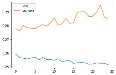
1
2
3
# loss crossentropy
model_loss = pd.DataFrame(model.history.history)
model_loss.plot()
1
<matplotlib.axes._subplots.AxesSubplot at 0x2a80381b2c8>
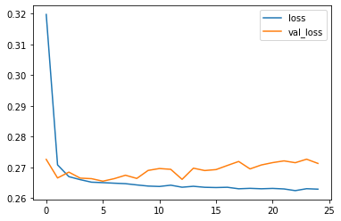
1
2
# predictions
predictions = model.predict_classes(X_test)
1
2
3
4
5
6
# metrics
print('\nConfusion Matrix:')
print(confusion_matrix(y_test,predictions))
print('\nClassification metrics:')
print(classification_report(y_test,predictions))
# non è fantastico perché la recall della classe 0 è bassa
1
2
3
4
5
6
7
8
9
10
11
12
13
Confusion Matrix:
[[ 7176 8482]
[ 406 62980]]
Classification metrics:
precision recall f1-score support
0 0.95 0.46 0.62 15658
1 0.88 0.99 0.93 63386
accuracy 0.89 79044
macro avg 0.91 0.73 0.78 79044
weighted avg 0.89 0.89 0.87 79044
New data prediction
1
2
3
4
5
# df
rn.seed(101)
random_ind = rn.randint(0,len(df))
new_customer = df.drop('loan_repaid',axis=1).iloc[random_ind]
new_customer
1
2
3
4
5
6
7
8
9
10
11
12
loan_amnt 25000.00
term 60.00
int_rate 18.24
installment 638.11
annual_inc 61665.00
...
zip_code_48052 0.00
zip_code_70466 0.00
zip_code_86630 0.00
zip_code_93700 0.00
earliest_cr_year 1996.00
Name: 305323, Length: 78, dtype: float64
1
2
3
4
5
6
# scaling
new_customer = scaler.transform(new_customer.values.reshape(1, 78))
# predict
print('Probabilità Prevista:', model.predict(new_customer))
print('Classe Prevista:', model.predict_classes(new_customer))
print('Classe Osservata:', df.iloc[random_ind]['loan_repaid'])
1
2
3
Probabilità Prevista: [[0.54277164]]
Classe Prevista: [[1]]
Classe Osservata: 1.0
1
2
# reset
%reset -f